Multilayer Perceptron in Machine Learning

Summary: Multilayer Perceptron in machine learning (MLP) is a powerful neural network model used for solving complex problems through multiple layers of neurons and nonlinear activation functions. This blog covers MLP’s architecture, forward and backward propagation, training methods, applications, and its pros and cons in Artificial Intelligence.

Introduction to Multilayer Perceptron (MLP)

The Multilayer Perceptron in machine learning (MLP) stands as one of the most fundamental and widely used architectures in the field of artificial neural networks and deep learning. Inspired by the human brain’s interconnected network of neurons, an MLP is a class of feedforward artificial neural network that consists of at least three layers of nodes: an input layer, one or more hidden layers, and an output layer.

Unlike the simple perceptron, which can only solve linearly separable problems, the MLP’s use of multiple layers and nonlinear activation functions enables it to model complex, nonlinear relationships in data, making it a powerful tool for a wide range of Machine Learning tasks such as classification, regression, and pattern recognition.

Key Takeaways:

• MLP uses multiple layers to model complex nonlinear relationships in data effectively.
• Activation functions introduce nonlinearity, enabling MLP to solve diverse problems.
• Backpropagation optimizes weights by minimizing prediction errors through gradient descent.
• Proper hyperparameter tuning and regularization prevent overfitting and improve generalization.
• MLPs are versatile but computationally intensive and require careful design and training.

Architecture of a Multilayer Perceptron

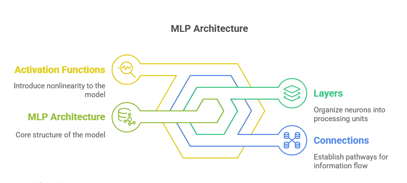
The architecture of an MLP is defined by its layers, the connections between neurons, and the activation functions that introduce nonlinearity into the model.

Layers in MLP

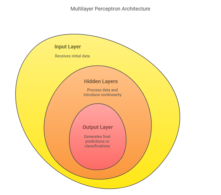
An MLP is composed of three main types of layers:

• Input Layer: This layer receives the raw input features from the dataset. Each neuron in the input layer represents a feature, and its sole purpose is to pass the input values to the next layer. No computation is performed at this stage.
• Hidden Layers: These are the core computational layers of the MLP. Each hidden layer consists of multiple neurons, and there can be one or more hidden layers in a network. 

Every neuron in a hidden layer receives input from all neurons in the previous layer (fully connected), applies a weighted sum and a bias, and passes the result through a nonlinear activation function. 

The presence of hidden layers allows the MLP to learn and represent complex patterns in the data.

• Output Layer: The final layer produces the output of the network, which could be a single value (for regression), a set of probabilities (for classification), or other forms depending on the task. The activation function used here depends on the nature of the problem—for example, softmax for multi-class classification or sigmoid for binary classification.

Neurons and Activation Functions

Each neuron in an MLP performs two main operations:

• Weighted Sum: The neuron computes a weighted sum of its inputs, adds a bias term, and then passes this sum through an activation function. Mathematically, for neuron jj in layer ll:

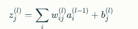
where wij(l)wij(l) is the weight connecting neuron ii in the previous layer to neuron jj in the current layer, ai(l−1)ai(l−1) is the activation from the previous layer, and bj(l)bj(l) is the bias.

• Activation Function: The activation function introduces nonlinearity, enabling the network to learn complex mappings. Common activation functions include:
  • Sigmoid: Squeezes input into the range (0, 1), useful for binary classification.
  • Tanh: Scales input to (-1, 1), often used in hidden layers.
  • ReLU (Rectified Linear Unit): Outputs zero for negative inputs and the input itself for positive values; popular due to its simplicity and effectiveness for deep networks.

How Multilayer Perceptron Works

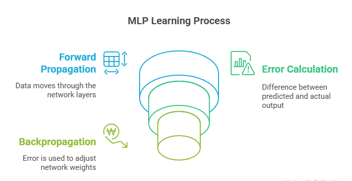
The functioning of an MLP can be understood through two main processes: forward propagation and backpropagation.

Forward Propagation

Forward propagation is the process by which input data is passed through the network to generate an output:

• The input features are fed into the input layer.
• Each subsequent layer computes a weighted sum of its inputs, adds a bias, and applies an activation function.
• This process continues layer by layer until the output layer produces the final prediction.

This step-by-step transformation allows the MLP to learn hierarchical representations of data, with each hidden layer extracting increasingly abstract features.

Backpropagation and Learning

Backpropagation is the learning algorithm that enables the MLP to adjust its weights and biases to minimize the error between its predictions and the actual target values:

• Loss Calculation: After forward propagation, the network’s output is compared to the true label using a loss function (e.g., mean squared error for regression, cross-entropy for classification).
• Gradient Computation: The gradients of the loss with respect to each weight and bias are computed using the chain rule of calculus. This process propagates the error backward through the network, hence the name “backpropagation”.
• Weight Update: The computed gradients are used to update the weights and biases using an optimization algorithm, typically stochastic gradient descent (SGD) or its variants. This iterative process continues for many epochs until the model converges to a set of parameters that minimize the loss.

Training a Multilayer Perceptron

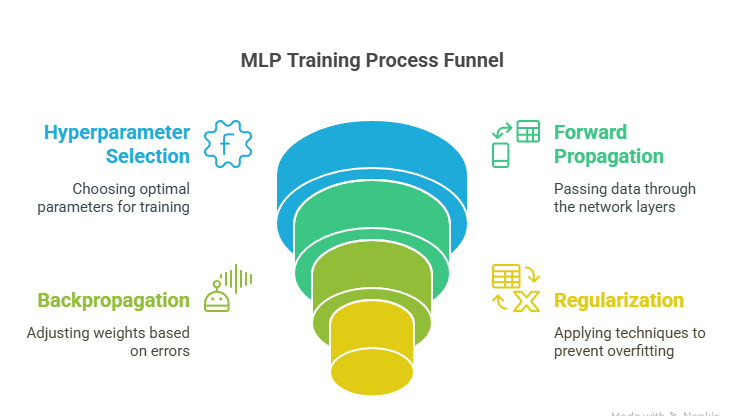
Training an MLP involves several critical steps and decisions that impact its performance.

Choosing Hyperparameters

Hyperparameters are settings that define the structure and learning process of the MLP. Key hyperparameters include:

• Number of Hidden Layers and Neurons: More layers and neurons increase the model’s capacity but also its risk of overfitting. The optimal architecture often requires experimentation and cross-validation.
• Learning Rate: Controls the size of the weight updates during training. A learning rate that is too high can cause the model to diverge, while a rate that is too low can result in slow convergence.
• Batch Size: Number of samples processed before the model’s internal parameters are updated. Smaller batch sizes can lead to noisier updates but may help escape local minima.
• Number of Epochs: The number of times the entire training dataset is passed through the network.
• Activation Functions: The choice of activation function can significantly affect learning dynamics and performance.

Regularization Techniques

Regularization methods help prevent overfitting, ensuring the MLP generalizes well to new data:

• L1 and L2 Regularization: Add a penalty to the loss function based on the magnitude of the weights, discouraging overly complex models.
• Dropout: Randomly disables a fraction of neurons during training, forcing the network to learn redundant representations and improving robustness.
• Early Stopping: Monitors performance on a validation set and stops training when performance ceases to improve, preventing overfitting.

Applications of Multilayer Perceptron

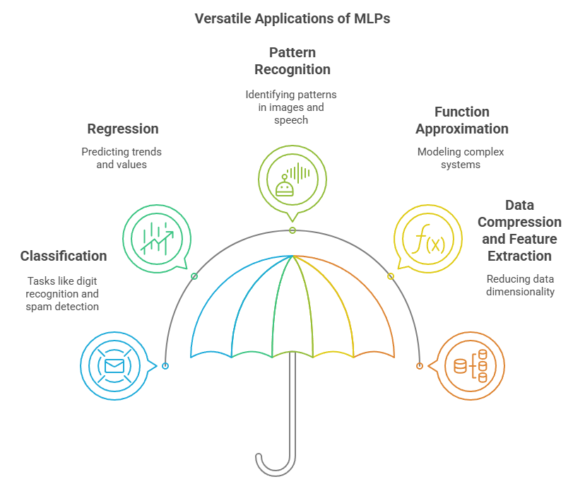
MLPs are highly versatile and have been successfully applied to a wide range of problems across industries:

• Classification: Handwritten digit recognition, spam detection, sentiment analysis, and medical diagnosis.
• Regression: Predicting house prices, stock market trends, and customer lifetime value.
• Pattern Recognition: Image and speech recognition, facial recognition, and object detection.
• Function Approximation: Modelling complex physical systems, financial forecasting, and control systems.
• Data Compression and Feature Extraction: Reducing dimensionality and extracting meaningful features from raw data for further processing.

Advantages and Limitations of MLP

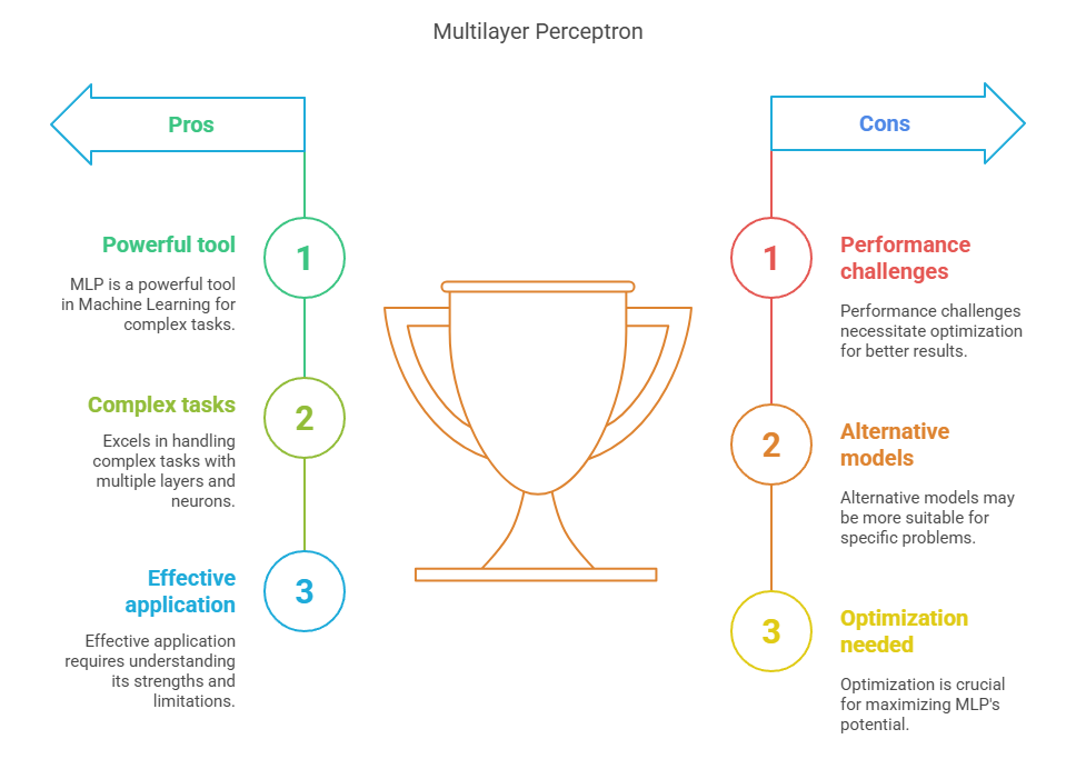
This section highlights both the strengths that make the multilayer perceptron a powerful tool in Machine Learning and the challenges it faces. Understanding these aspects is crucial for effectively applying MLPs, optimizing their performance, and knowing when alternative models might be more suitable.

Advantages

• Universal Approximation: MLPs can approximate any continuous function given sufficient neurons and data, making them highly flexible.
• Nonlinear Modelling: The use of nonlinear activation functions allows MLPs to capture complex relationships in data.
• Versatility: Applicable to a wide range of supervised learning tasks, including classification and regression.

Limitations

• Computational Complexity: Training deep MLPs can be computationally expensive and time-consuming, especially with large datasets.
• Overfitting: MLPs with too many parameters can easily overfit the training data, requiring careful regularization and validation.
• Lack of Interpretability: The internal representations learned by MLPs are often considered “black boxes,” making it difficult to interpret model decisions.
• Sensitivity to Hyperparameters: Performance is highly dependent on the choice of hyperparameters, requiring extensive tuning and experimentation.

Conclusion: Why MLP is Important in AI

The Multilayer Perceptron in machine learning is a foundational architecture in the field of Artificial Intelligence and Machine Learning. Its ability to learn complex, nonlinear relationships in data has made it a cornerstone of deep learning and a precursor to more advanced neural network architectures such as convolutional and recurrent neural networks.

Despite its limitations, the MLP remains a go-to model for many practical applications and serves as an essential stepping stone for anyone looking to understand and leverage the power of neural networks in AI

Frequently Asked Questions

What is the Main Difference Between a Perceptron and a Multilayer Perceptron?

A perceptron has a single layer and can only solve linearly separable problems. A multilayer perceptron contains one or more hidden layers with nonlinear activation functions, enabling it to solve complex, nonlinear problems by learning hierarchical data representations.

How Does Backpropagation Work in Training An MLP?

Backpropagation calculates the gradient of the loss function with respect to each weight by propagating errors backward through the network. These gradients are used to update weights via optimization algorithms like gradient descent, minimizing prediction errors iteratively.

What Are Common Activation Functions Used in Mlps and Why?

Common activation functions include ReLU, sigmoid, and tanh. ReLU is popular for hidden layers due to efficient gradient flow and simplicity. Sigmoid and tanh are used for output layers or specific tasks, introducing nonlinearity and enabling the network to model complex patterns.