Regression in Machine Learning: Types & Examples

Summary: This blog explores regression in machine learning, detailing various types, such as linear, polynomial, and ridge regression. It explains when to use each model and their applications for predicting continuous outcomes.

Introduction

Machine Learning has become a fundamental part of people’s lives, and it typically has two segments: supervised and unsupervised learning. Supervised Learning deals with labelled data, and unsupervised learning deals with unlabelled data. 

Supervised learning can be classified into classification and regression, where regression deals with continuous values and the former deals with discrete values. The following blog revolves around Regression in Machine Learning and its types. 

What is Regression in ML? 

Regression Machine Learning algorithms are a statistical method for modelling the relationship between dependent variables and one or more independent variables. The analysis helps you understand the change in the value of the target variable corresponding to an independent variable. 

It is possible when the other independent variables are held at a fixed value. There are different types of regression in Machine Learning Regression algorithms, where the target variable with continuous values and independent variables show a linear or non-linear relationship. 

Effectively, regression algorithms help determine the best-fit line. It passes through all data points in a way that the distance of the line from each data point is minimal.

15 Types of Regression Models & when to use them

Regression algorithm models are statistical techniques used to model the relationship between one or more independent variables (predictors) and a dependent variable (response). There are various regression models in ML, each designed for specific scenarios and data types. Here are 15 types of regression models and when to use them:

Linear Regression 

Linear regression is used when the relationship between the dependent and independent variables is assumed to be linear. It is suitable for continuous numerical data and when a straight line can predict the response variable.

Linear regression is a fundamental and widely used statistical method for modelling the relationship between a dependent variable (Y) and one or more independent variables (X). 

It assumes a linear relationship between the predictor(s) and the response variable. Mathematically, a simple linear regression can be expressed as Y = β0 + β1*X + ε, where β0 and β1 are the coefficients and ε represents the error term.

Example: Suppose we want to predict house prices (Y) based on their size (X). We collect data on various houses, their respective sizes, and their actual selling prices. The goal is to fit a straight line that best describes the relationship between house size and price.

Multiple Linear Regression 

It is similar to linear regression, but it involves multiple independent variables. It is used when the response variable depends on more than one predictor variable.

Multiple linear regression extends the concept of simple linear regression to include more than one independent variable. The model becomes Y = β0 + β1X1 + β2X2 + … + βn*Xn + ε, where n is the number of predictors.

Example: Building on the house price prediction example, we can include additional features such as the number of bedrooms, location, and house age. The multiple linear regression model will help us understand how each predictor contributes to the overall price prediction.

Polynomial Regression 

Polynomial regression is used when a polynomial function rather than a straight line can better approximate the relationship between the dependent and independent variables. It is suitable when data follows a curvilinear pattern.

Sometimes, the relationship between the predictors and the response variable may not be linear. Polynomial regression allows us to capture more complex patterns by using polynomial functions of the predictors (X). The model can be expressed as: Y = β0 + β1X + β2X^2 + … + βn*X^n + ε.

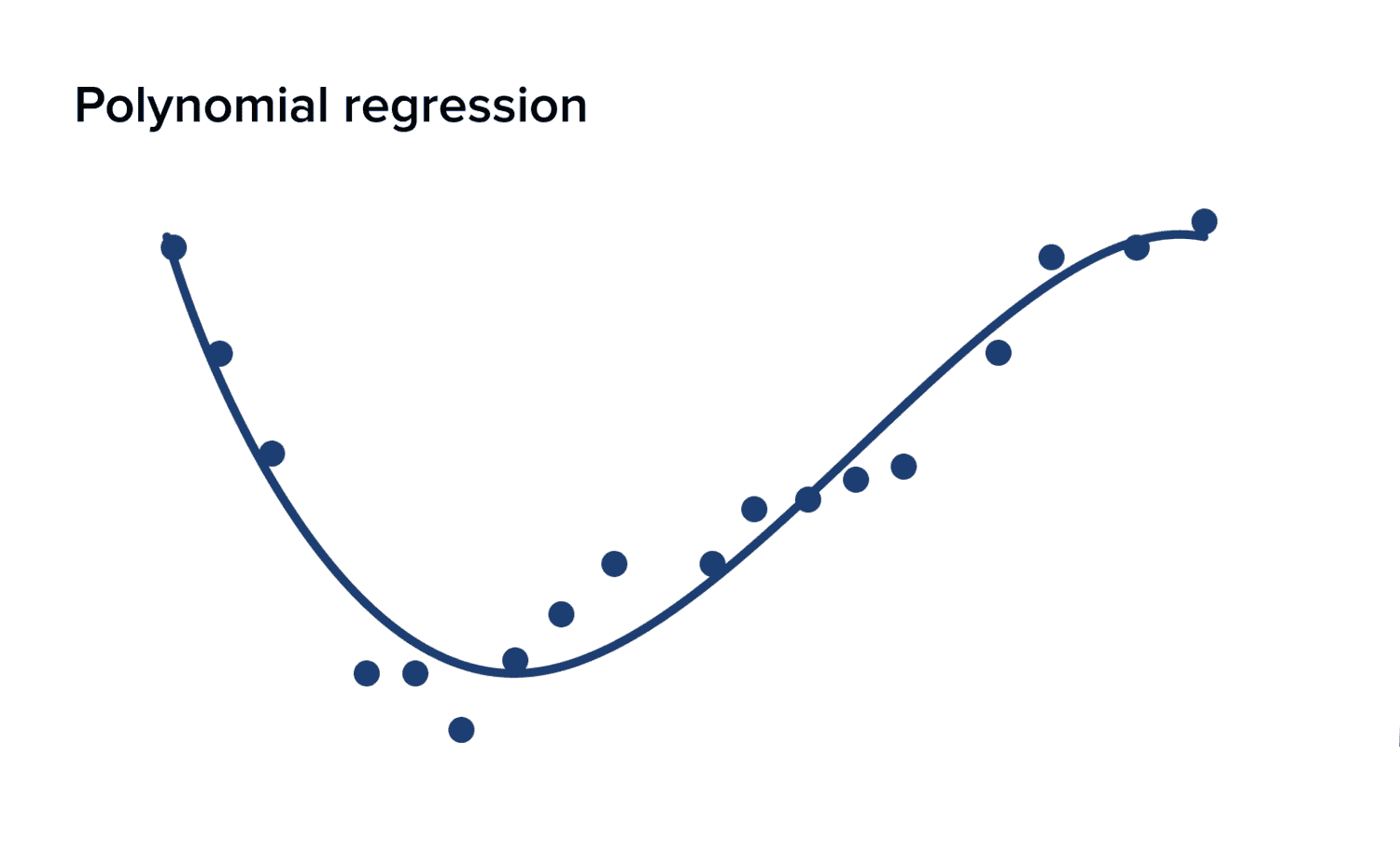
Example: Consider the temperature and gas consumption example. If gas consumption increases with temperature nonlinearly, polynomial regression can help us model this relationship more accurately.

Ridge Regression (L2 Regularisation)

In multiple linear regression, ridge regression is used to handle multicollinearity (high correlation between predictors). It stabilises the model by adding a penalty term to the least squares objective function.

Ridge regression is a regularised linear regression that addresses multicollinearity issues (high correlation between predictors). It adds a penalty term (L2 norm) to the least squares objective function, which prevents large coefficient values. This regularisation helps to stabilise the model and reduces overfitting.

Example: In a sales prediction scenario, advertising expenses and promotion budgets might be highly correlated. Ridge regression can be used to prevent overemphasising one of these variables and achieve a more robust model.

Lasso Regression (L1 Regularisation) 

Lasso regression is used when you want to perform feature selection along with regression. It adds an absolute value penalty term to the least squares objective function, forcing some coefficients to become precisely zero.

Lasso regression is another regularisation technique used for feature selection along with regression. It adds an absolute value penalty term (L1 norm) to the least squares objective function. This causes some coefficients to become exactly zero, effectively performing variable selection.

Example: In a medical study, several potential predictors of disease occurrence exist. Lasso regression can help identify the most relevant predictors and eliminate the less important ones.

6. Decision Tree Regression: 

Decision tree regression is a non-parametric Machine Learning technique for predicting continuous values. It constructs a tree-like structure by recursively splitting the data based on feature values, creating branches and leaf nodes. 

Each leaf node represents a predicted value for the target variable. The algorithm is simple to interpret and can capture complex relationships in the data.

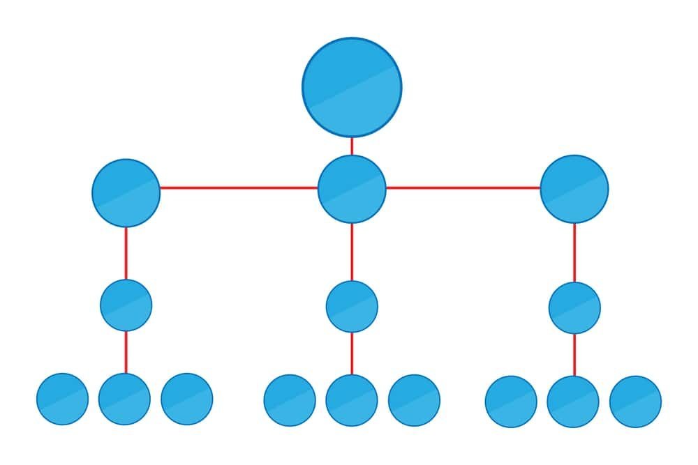
Example: Suppose we have a dataset containing information about houses, including their size, number of bedrooms, and sale prices. We want to use decision tree regression to predict the cost of a new home based on its features.

The decision tree algorithm analyses the data and creates a tree structure. First, the data might be split based on the size of the house. If the home is smaller than a certain threshold, it goes to the left branch; if it’s larger, it goes to the right branch. Then, the data is split further based on the number of bedrooms.

Read Blog: A tale of regression and regressiveness

Logistic Regression 

Logistic regression is a powerful statistical method designed for binary classification tasks, where the goal is to predict one of two possible outcomes, such as yes/no or true/false. This technique models the probability of a specific outcome occurring by applying a logistic (or sigmoid) function to a linear combination of predictor variables. 

By transforming these predictors through the logistic function, the model outputs a probability that ranges between 0 and 1. This allows it to estimate the likelihood of the binary response, making logistic regression a crucial tool for decision-making in scenarios where outcomes are categorical and mutually exclusive.

Example: In email spam classification, logistic regression can predict the probability that an email is spam based on various email features.

Poisson Regression 

Poisson regression is a statistical technique design for modelling count data, where the dependent variable represents the number of occurrences of an event within a fixed period. This method is particularly useful when the data follows a Poisson distribution, which describes the probability of a given number of events happening within a fixed interval. 

Unlike other regression models, Poisson regression assumes that the mean rate of occurrence is equal to the variance, making it suitable for data with low to moderate event counts. Analysts can effectively predict and interpret the relationship between count data and independent variables by applying Poisson regression, offering insights into event patterns and rates.

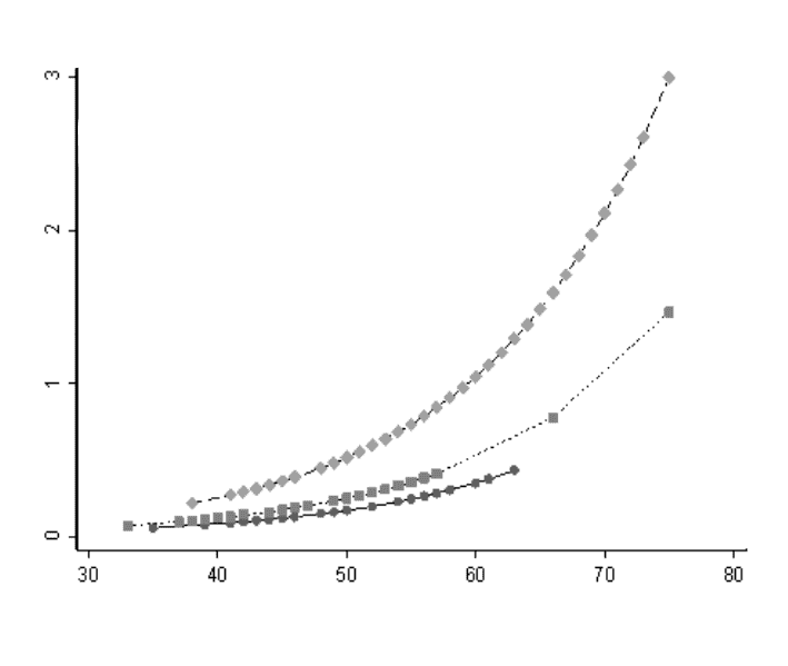
Example: Modeling the number of customer service calls a company receives daily based on factors like day of the week, advertising campaigns, or seasonal effects.

Negative Binomial Regression

Negative binomial regression builds on Poisson regression to address overdispersion in count data. While Poisson regression assumes that the variance equals the mean, negative binomial regression allows for greater flexibility by introducing an additional parameter to account for overdispersion. This extra parameter captures the variability in the data that Poisson regression cannot handle. 

As a result, negative binomial regression provides a more accurate model for datasets where the variance exceeds the mean, making it especially useful for analysing count data with high variability. Accommodating this extra dispersion offers a more robust and reliable analysis of count outcomes.

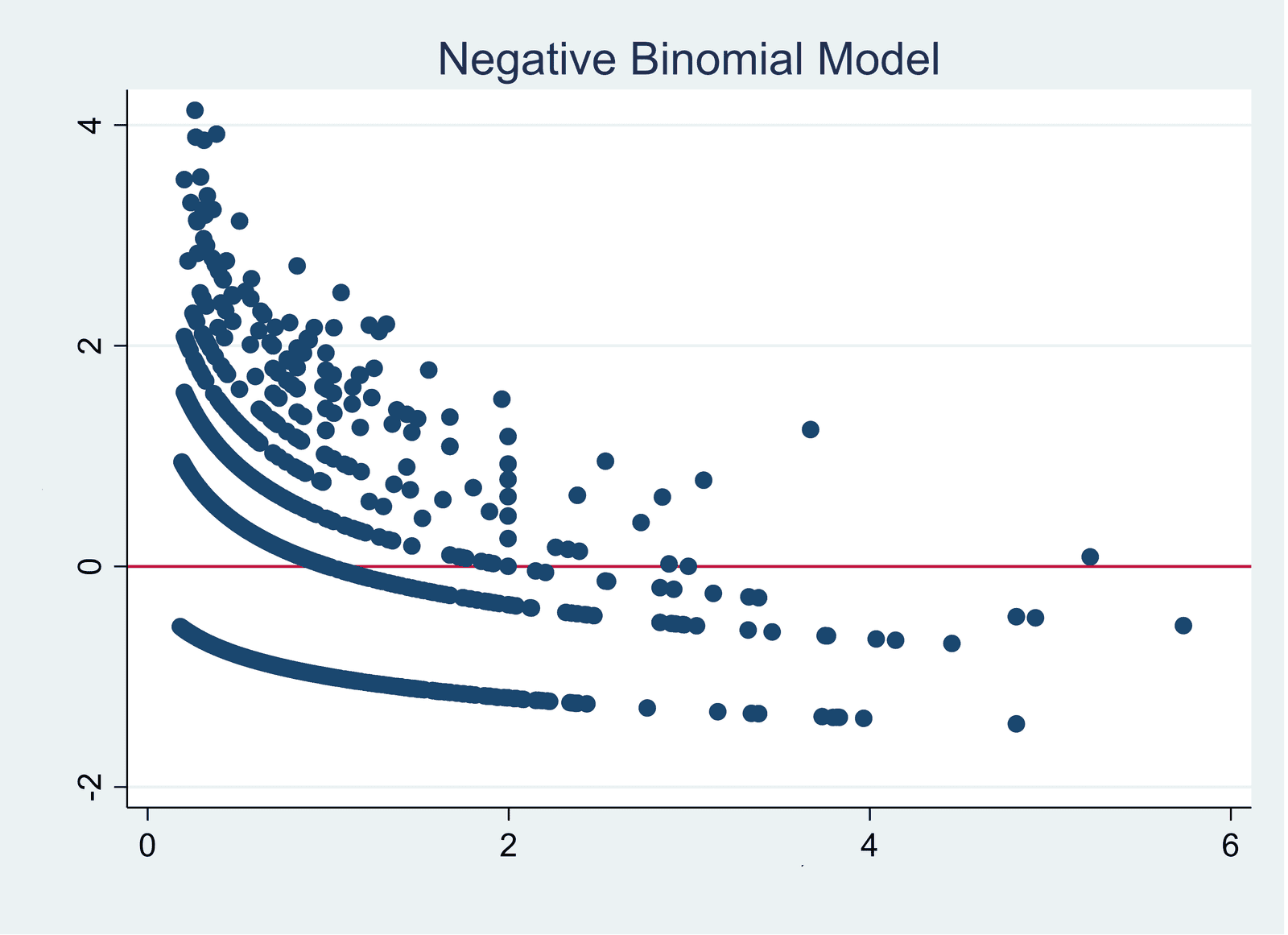
Example: Predicting the number of accidents in a factory per day, where the count data might show more variation than expected from a simple Poisson model.

Cox Regression (Proportional Hazards Model) 

Cox regression, also known as the Proportional Hazards Model, is a key statistical method in survival analysis. It examines the impact of predictor variables on the time until an event occurs, such as patient survival time in medical studies. 

This model is precious in clinical research, where it helps to identify how different factors, like treatments or demographics, influence the risk of an event over time. 

By estimating hazard ratios, Cox regression allows researchers to understand and quantify the relationship between covariates and the hazard of experiencing the event, providing critical insights for decision-making and prognosis.

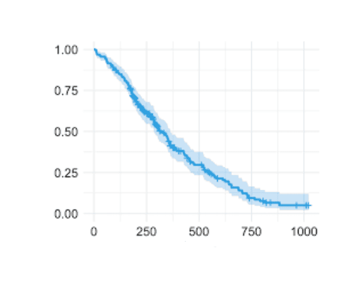
Example: Analysing the impact of different treatments on the survival time of cancer patients after diagnosis.

Stepwise Regression

Stepwise regression is a statistical technique to build efficient and simplified models by selecting the most significant predictor variables from a more extensive set. This method systematically adds or removes variables based on their contribution to the model’s predictive power. Initially, it starts with no variables in the model or a subset of predictors. 

It then evaluates the impact of adding each variable, selecting those that improve the model’s performance. Conversely, it may also remove variables that no longer contribute meaningfully. This iterative process helps create a model that balances complexity and accuracy, including only the most relevant predictors.

Example: Selecting the most important features from a large dataset to predict the market performance of a particular product.

Time Series Regression

Time series regression is employe when analysing data points collected or recorded at successive intervals. This method focuses on understanding how the dependent variable, a time series, is influenced by its previous values or lagged observations. 

In other words, it examines how past values of the dependent variable and different independent variables impact its future values. By incorporating lagged variables into the model, time series regression helps capture patterns and trends over time, allowing for better predictions and insights into temporal dynamics within the data.

Example: Predicting a company’s stock prices based on its past stock prices and economic indicators.

Explore: Demystifying Time Series Database: A Comprehensive Guide.

Panel Data Regression (Fixed Effects and Random Effects Models) 

Panel data regression is a powerful analytical technique used when researchers collect data from multiple entities over time. This method allows for controlling individual-specific effects, which are constant over time but vary between entities, through fixed-effects models. 

By focusing on within-entity variations, fixed-effects models help isolate and analyse the influence of variables unique to each entity. Alternatively, random effects models account for random variations across entities and assume these effects are uncorrelated with the explanatory variables. 

This approach is beneficial when the variability is more general and less specific to each entity. Together, these models provide robust insights into temporal and entity-specific dynamics.

Example: Analysing the impact of educational policies on students’ test scores across different schools over several years.

Bayesian Regression

Bayesian regression is a powerful technique incorporating prior knowledge or beliefs about model parameters into the regression analysis. Unlike traditional regression methods that yield point estimates, Bayesian regression offers a probabilistic framework, allowing you to understand the uncertainty around predictions. 

This approach combines prior distributions, representing your initial beliefs about the parameters, with the likelihood of the observed data. 

As a result, Bayesian regression provides a range of possible values for the parameters rather than a single estimate, which helps make more informed decisions under uncertainty. This method is beneficial when dealing with complex models or limited data.

Example: Estimating the demand for a product based on past sales data while incorporating prior knowledge about similar products and market trends.

Quantile Regression

Quantile regression is a statistical technique that models the relationship between predictors and various quantiles of the dependent variable. Unlike ordinary least squares regression, which focuses solely on the mean of the response variable, quantile regression provides insights into different points of the conditional distribution. 

Analysing different quantiles, such as the median or the 90th percentile, offers a richer understanding of how predictors influence the entire distribution of the outcome variable. This method is handy when the data exhibits heteroscedasticity or when outliers might disproportionately affect the mean, allowing for a more nuanced view of the data’s variability.

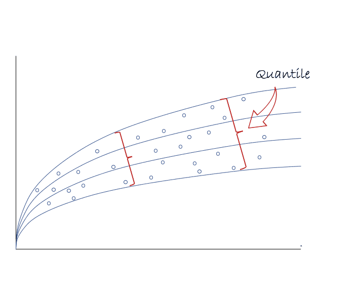
Example: Studying the relationship between weather variables and electricity consumption at various quantiles to understand the impact on different demand levels.

The choice of regression model depends on the nature of your data, the assumptions of the relationship between variables, the type of dependent variable, and your specific research or prediction objectives. Always validate the chosen model’s assumptions and assess its performance using appropriate evaluation metrics before concluding the results.

Frequently Asked Questions

What is a regression in machine learning?

Regression in machine learning is a statistical method for modelling the relationship between a dependent variable and one or more independent variables. It aims to predict continuous outcomes by finding the best-fit line or curve through data points, minimising the distance between the line and actual data.

When should I use polynomial regression?

Use polynomial regression when the relationship between your variables is not linear. It extends linear regression by fitting a polynomial function to the data, which can capture more complex, curvilinear relationships and provide a better model for datasets with non-linear patterns.

What is the difference between ridge and lasso regression?

Ridge regression adds an L2 penalty to the regression model to handle multicollinearity and stabilise coefficients. Lasso regression adds an L1 penalty, which can shrink some coefficients to zero, effectively performing feature selection. Ridge is for multicollinearity, while Lasso is for feature reduction.

Conclusion

From the above blog, you have learned about Regression Algorithms in Machine Learning. A regression-supervised learning technique helps find correlations between variables. It enables you to predict the continuous output variable based on one or more predictor variables. 

Join Pickl.AI for its range of Data Science courses, including Machine Learning and Supervised Learning. You’ll be able to develop your skills and expertise in regression effectively.