Aging Formula in Excel – A Step-by-Step Guide for Beginners and Professionals

Summary: Learn the aging formula in Excel using TODAY() and DATEDIF() to calculate item age. This guide covers creating aging buckets (0-30, 31-60 days) with IF/VLOOKUP, building AR reports, and best practices for effective financial tracking and inventory management.

Introduction

In the fast-paced world of business, keeping track of outstanding items – be it invoices, inventory, or tasks – is crucial for financial health and operational efficiency. One of the most effective ways to do this is through an “aging analysis.” Excel, with its powerful formula capabilities, provides an excellent platform for creating dynamic aging reports.

This guide will walk you through everything from the basic concepts to building a practical accounts receivable aging report, catering to both Excel novices and seasoned professionals looking for a refresher or new tricks.

Key Takeaways

• Use TODAY() and DATEDIF() to accurately calculate item age in days.
• Categorize ages into buckets using IF, IFS, or VLOOKUP for clarity.
• Build Accounts Receivable aging reports to effectively track overdue payments.
• Leverage Excel Tables (Ctrl+T) for dynamic, easy-to-manage aging data.
• Summarize aging data with PivotTables or SUMIF(S) for quick insights.

What is an Aging Formula in Excel?

At its core, an aging formula in Excel calculates the duration an item has been outstanding or in a particular state. For instance:

• Accounts Receivable (AR): How long has an invoice been unpaid since its due date?
• Accounts Payable (AP): How long until an invoice is due, or how overdue is a payment?
• Inventory Management: How long has a product been sitting in the warehouse?
• Task Management: How long has a task been open or past its deadline?

The “formula” part refers to the specific Excel functions used to determine this time difference, typically between a start date (e.g., invoice date, received date) and a reference date (usually today’s date or a specific reporting date). The output is often expressed in days, which can then be categorized into “aging buckets” (e.g., 0-30 days, 31-60 days) for easier analysis and prioritization.

The primary purpose of an aging analysis is to provide visibility. For AR, it helps identify overdue payments, assess credit risk, and guide collection efforts. For inventory, it can flag slow-moving or obsolete stock, informing purchasing and sales strategies.

Basic Aging Formula Using TODAY() and DATEDIF

Let’s start with the fundamentals. To calculate the age of an item as of the current date, we primarily use two Excel functions: TODAY() and DATEDIF().

TODAY() Function

This simple function returns the current date. It’s dynamic, meaning it updates every time the workbook is opened or recalculated.

• Syntax: =TODAY()

DATEDIF() Function

This powerful function calculates the difference between two dates in various units (days, months, years).

• Syntax: =DATEDIF(start_date, end_date, unit)
  • start_date: The earlier date (e.g., invoice date).
  • end_date: The later date (e.g., TODAY()).
  • unit: The unit of time you want the result in:
    • “d”: Difference in total days.
    • “m”: Difference in complete months.
    • “y”: Difference in complete years.
    • “ym”: Difference in months, ignoring years.
    • “yd”: Difference in days, ignoring years.
    • “md”: Difference in days, ignoring months and years.

Example: Calculating the Age of an Invoice in Days

Suppose you have an invoice date in cell A2. To find out how many days old this invoice is as of today:

1. Invoice Date (Cell A2): 01/15/2024 (ensure this is formatted as a date)
2. Aging Formula (Cell B2): =DATEDIF(A2, TODAY(), “d”)

If today is 03/25/2024, the formula in cell B2 would return 70 (representing 70 days).

Important Note on DATEDIF

For DATEDIF to work correctly, the start_date must be earlier than or equal to the end_date. If start_date is later, DATEDIF will return a #NUM! error. You can wrap this in an IFERROR function or an IF statement to handle such cases (e.g., for items not yet due).
Example: =IF(A2>TODAY(), 0, DATEDIF(A2, TODAY(), “d”)) – this would show 0 days if the invoice date is in the future.

For calculating “days overdue” based on a due date rather than an invoice date, the logic is similar. If the due date is in cell C2:
=IF(TODAY()>C2, TODAY()-C2, 0)
This formula calculates the number of days past the due date. If it’s not yet due, it returns 0. Format this cell as a “General” or “Number” to see the day count.

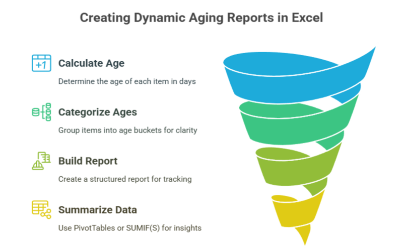
Creating an Aging Bucket in Excel

Simply knowing the number of days an item is aged is useful, but categorizing these ages into “buckets” provides a more structured view for reporting and decision-making. Common buckets for AR include:

• Current (or 0-30 days)
• 31-60 days
• 61-90 days
• 91-120 days
• Over 120 days

We can use nested IF statements or the IFS function (available in newer Excel versions) to assign an item to a bucket based on its age in days.

Let’s assume the “Age in Days” calculated in the previous step is in cell B2.

Using Nested IF Statements (Cell C2)

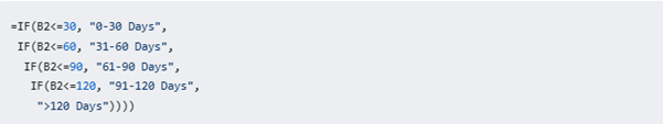
Explanation:

• The formula checks conditions sequentially.
• If B2 (Age in Days) is less than or equal to 30, it returns “0-30 Days.”
• If not, it checks if B2 is less than or equal to 60, returning “31-60 Days,” and so on.
• The final “>120 Days” acts as the catch-all for anything older.

Using IFS Function (Cell C2 – for Excel 2019, Microsoft 365 and later)

The IFS function can be cleaner for multiple conditions

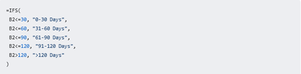
Here, B2>120 is explicitly stated, which is good practice. You could also use TRUE as the last condition in IFS to act as a catch-all: TRUE, “>120 Days”.

Alternative: Using VLOOKUP with a Helper Table (More Scalable)

For many buckets or if you want to easily change bucket definitions, VLOOKUP with TRUE (approximate match) is excellent.

Create a Helper Table (e.g., on a separate sheet or an unused area, say F1:G5):

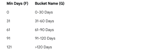
Important: The first column of the lookup table (Min Days) must be sorted in ascending order.

VLOOKUP Formula (Cell C2)

1. • B2: The age in days you want to look up.
   • $F$1:$G$5: The absolute reference to your helper table.
   • 2: Return the value from the second column of the helper table (Bucket Name).
   • TRUE: Finds an approximate match. It looks for the largest value in the first column of the lookup table that is less than or equal to the lookup value (B2).

This VLOOKUP method is more flexible if your bucket definitions change frequently.

Accounts Receivable Aging Report Template in Excel

Now, let’s combine these concepts to build a basic Accounts Receivable (AR) Aging Report.

Typical Columns for an AR Aging Report:

1. Invoice Number: (e.g., INV-001)
2. Customer Name: (e.g., Acme Corp)
3. Invoice Date: (e.g., 01/01/2024)
4. Due Date: (Calculated or entered. E.g., If payment terms are Net 30, Due Date = Invoice Date + 30 days)
5. Invoice Amount: (e.g., $1500)
6. Days Overdue: (Calculated: MAX(0, TODAY() – DueDateCell))
7. Aging Bucket: (Calculated using IF/IFS or VLOOKUP based on “Days Overdue”)

Example Setup:

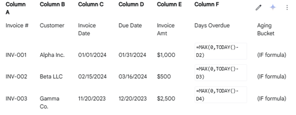
• Cell D2 (Due Date example, assuming Net 30): =C2+30 (drag down)
• Cell F2 (Days Overdue): =MAX(0,TODAY()-D2) (drag down). MAX(0, …) ensures no negative days if it’s not yet due.
• Cell G2 (Aging Bucket, using IFS on Days Overdue in F2):

• (Adjust buckets as needed; “Current” for 0 days overdue, then “1-30”, etc.)

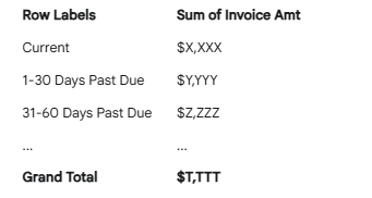
Summarizing the Report

Once you have this detailed list, you’ll want to summarize the total amounts in each aging bucket. A PivotTable is ideal for this:

1. Select your entire data range (A1 to Gx).
2. Go to Insert > PivotTable.
3. Choose where to place the PivotTable (New Worksheet or Existing Worksheet).
4. In the PivotTable Fields pane:
   • Drag “Aging Bucket” to the Rows area.
   • Drag “Invoice Amount” to the Values area (it should default to Sum of Invoice Amount).
5. You’ll get a neat summary:

Alternatively, you can use SUMIF or SUMIFS functions if you prefer a static summary table. For example, to sum amounts for “1-30 Days Past Due”:

=SUMIF(G:G, “1-30 Days Past Due”, E:E)

Tips and Best Practices

Now that you grasp the basics, let’s refine your approach. This “Tips and Best Practices” section offers actionable advice to enhance accuracy, improve efficiency, and build more robust Excel aging reports, ensuring clearer and more reliable financial insights.

• Consistent Date Formats: Ensure all your date columns are actually formatted as dates in Excel, not text. Inconsistent formats are a common source of errors.
• Helper Columns: Don’t be afraid to use them! Calculating “Days Overdue” in one column and then using that result for the “Aging Bucket” in another makes formulas easier to build, read, and debug.
• Use Excel Tables (Ctrl+T): Convert your data range into an Excel Table. This provides structured references (e.g., Table1[DueDate]), which are more readable, and formulas automatically fill down when you add new rows.
• Named Ranges: For lookup tables or key cells (like a report date if not TODAY()), define named ranges (Formulas > Define Name) for better readability and easier maintenance.
• Conditional Formatting: Use conditional formatting to visually highlight rows based on their aging bucket (e.g., color-code severely overdue invoices red).
• Error Handling: Use IFERROR to gracefully handle potential errors, especially with DATEDIF if start dates might be after end dates, or if dates are missing.

Example: =IFERROR(DATEDIF(A2,TODAY(),”d”), “Invalid Date”)

Dynamic Reporting Date: If you don’t want to use TODAY() and prefer a fixed reporting date (e.g., month-end), put that date in a specific cell and reference it in your formulas instead of TODAY().

Clarity in Buckets: Ensure your bucket logic is clear and covers all possibilities without overlaps (unless intended for some specific reason). The VLOOKUP method helps avoid logical errors in complex nested IFs.

Conclusion: Beyond Basic Excel – When to Consider More

Excel is incredibly versatile for creating aging reports, especially for small to medium-sized datasets and standard requirements. The TODAY(), DATEDIF(), IF/IFS, and VLOOKUP functions, combined with PivotTables, provide a robust toolkit for insightful aging analysis across various business functions. 

From basic invoice aging to tracking inventory freshness, the principles remain the same: calculate the time difference and categorize it.

However, as data volumes grow substantially or reporting needs become highly complex and specific to regulatory frameworks (e.g., nuanced inventory valuation methods in pharmaceuticals, or sophisticated credit risk modeling for large financial institutions), the limitations of a pure Excel-formula-based approach might surface. 

Performance can degrade with tens of thousands of rows involving complex array formulas or volatile functions. Maintaining consistency across multiple users without robust version control can also be challenging.

In such scenarios, while Excel can still serve as a front-end reporting tool, it’s often beneficial to consider industry-specific software, Enterprise Resource Planning (ERP) systems with built-in aging modules, or dedicated Business Intelligence (BI) platforms. These tools are designed for larger datasets, offer more sophisticated analytics, ensure data integrity, and often come with pre-built reporting tailored to specific industry needs. 

They can handle the heavy lifting of data processing, allowing Excel to be used for final presentation or ad-hoc analysis if needed. The choice depends on your organization’s scale, complexity, and specific industry requirements.

Frequently Asked Questions

My DATEDIF Formula Shows a #NUM! Error. What is Wrong?

This usually means your start_date is later than your end_date. DATEDIF requires the start date to be earlier. Double-check your dates or use an IF statement to handle cases where items are not yet “aged” (e.g., future due dates).

How Can I Create Aging Buckets for Items That Aren’t Due Yet (e.g., “Due in 0-30 days”)?

You’d calculate the difference between the DueDate and TODAY(). If DueDate is in A2: =A2-TODAY() will give days remaining. Then use IF/IFS to categorize: IF(A2-TODAY()<=30, “Due in 0-30 Days”, …) for positive results.

Can I Make My Aging Report Update Automatically Without Opening the File?

Excel formulas with TODAY() update when the file is opened or recalculated. For fully automated, server-side updates feeding into a dashboard, you’d typically look into Power BI with scheduled refreshes, or scripts (like Python) running on a server to process data and update a source.