How to Freeze a Row in Excel: Step-by-Step Guide

Summary:  Freezing a row in Excel is easy. All you need to know is the right steps to follow. This blog unfolds the key steps to freeze a row. The process is simple and includes: Select View > Freeze Panes > Freeze Panes.

Introduction

Excel spreadsheets can be vast, often stretching far beyond the visible screen. Although there are several Excel formulas to simplify the task, when you’re scrolling through hundreds or even thousands of data entries, it’s incredibly frustrating to lose sight of your column headers.

How do you remember what each number or text string refers to? The answer lies in a handy feature called “Freeze Panes.” This guide will walk you through everything you need to know about how to freeze a row in Excel, ensuring your headers are always in view.

What Does Freezing a Row in Excel Mean?

When you “freeze” a row (or multiple rows) in Excel, you’re essentially locking them into place at the top of your worksheet. This means that no matter how far down you scroll, the frozen rows will remain visible, acting as a constant reference point for your data. 

It is an indispensable tool for data analysis, data entry, and anyone who frequently works with large datasets. Think of it as putting a thumbtack in your header row so it doesn’t move.

Steps to Freeze the Top Row in Excel

Why would you want to freeze just the top row? Because it’s the most common scenario where your column headers reside!

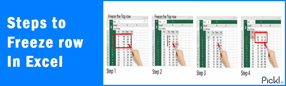
Step 1: Open Your Worksheet: Launch Excel and open the spreadsheet where you want to freeze the top row.

Step 2: Navigate to the View Tab: In the Excel ribbon at the top of your screen, click on the “View” tab.

Step 3: Locate Freeze Panes: Within the “View” tab, in the “Window” group, you’ll find a button labelled “Freeze Panes.” Click on it.

Step 4: Select “Freeze Top Row”: From the dropdown menu that appears, choose the option “Freeze Top Row.”

That’s it! You’ll notice a subtle line appearing below your first row, indicating it’s now frozen. Scroll down, and your top row will stay put!

Read more about conditional formatting in Excel

How to Freeze Any Row in Excel (Not Just the Top Row)

When do you need to freeze a row that isn’t the first one? Perhaps your data starts after a few title rows, or you want to keep a specific set of information visible.

To freeze a row other than the very top one, you need to select the row below the one you want to freeze. Excel freezes everything above your selection.

Step 1: Click on the Row Header: If you want to freeze up to Row 5, for example, click on the row header (the number 6) for Row 6. This selects the entire row.

Step 2: Go to the View Tab: Click on the “View” tab in the Excel ribbon.

Step 3: Click “Freeze Panes”: In the “Window” group, click the “Freeze Panes” button.

Step 4: Choose “Freeze Panes”: From the dropdown, select the first option, simply labeled “Freeze Panes.”

Now, all rows from Row 1 up to (and including) Row 5 will be frozen. When you scroll, they’ll remain visible.

Shortcut to Freeze Rows in Excel

How do you quickly freeze rows without all the clicking? While there isn’t a single direct keyboard shortcut for “Freeze Top Row,” you can navigate to the “Freeze Panes” menu using hotkeys:

Step 1: Press Alt. (You’ll see letters appear on the ribbon tabs.)

Step 2: Press W (for View tab).

Step 3: Press F (for Freeze Panes).

Step 4: Then, press R (for Freeze Top Row) or F again (for Freeze Panes, if you’ve selected a row).

This method requires a few key presses but can be faster once you get the hang of it.

How to Unfreeze Rows in Excel

What if you no longer need rows frozen, or you want to change which rows are frozen? Unfreezing is just as simple.

Step 1: Go to the View Tab: Click on the “View” tab in the Excel ribbon.

Step 2: Click “Freeze Panes”: In the “Window” group, click the “Freeze Panes” button.

Step 3: Select “Unfreeze Panes”: From the dropdown menu, choose the option “Unfreeze Panes.”

All previously frozen rows will now be unfrozen, and your worksheet will scroll normally.

Difference Between Freeze Row, Freeze Column, and Split

Understanding the difference between Freeze Row, Freeze Column, and Split is essential for efficiently viewing and analyzing data in Excel. These features allow users to keep key headers visible or create separate worksheet areas, enhancing navigation and comparison across large datasets while working with complex spreadsheets.

Freeze Top Row

As discussed, this locks the very first row of your worksheet.

Freeze First Column

This locks the very first column of your worksheet (Column A). Useful if you have important identifiers in that column that you always want to see when scrolling horizontally.

Freeze Panes

This is the most versatile option. It freezes all rows above your current cell selection and all columns to the left of your current cell selection. For example, if you select cell C4 and then choose “Freeze Panes,” rows 1-3 and columns A-B will be frozen. This is how you freeze multiple rows and/or multiple columns simultaneously.

Split

This creates separate scrollable regions within your worksheet. Unlike freezing, which keeps a section fixed, splitting allows you to scroll independently in different parts of the same sheet. It’s helpful for comparing data in different sections without freezing any headers.

Common Issues & Fixes

Why aren’t my freeze panes working? If you are still wondering, then here are some of the common reasons responsible for frozen panes.

“Freeze Panes” is grayed out

This often happens if you are in “Page Break Preview” or “Page Layout View.” Switch back to “Normal View” (found on the “View” tab) and try again.

Only one row/column is freezing when I want more

Remember, if you use “Freeze Top Row” or “Freeze First Column,” it will only freeze that single row or column. To freeze multiple rows, select the row below where you want the freeze line, then use the generic “Freeze Panes” option.

I froze the wrong section

Simply “Unfreeze Panes” and then re-apply the freeze to the correct section.

My data is overlapping the frozen pane

Ensure your frozen rows are tall enough to display all content, or wrap text within those cells if necessary.

Frequently Asked Questions

How do I freeze specific rows in Excel?

To freeze specific rows (e.g., rows 1-5), click on the row header for the row immediately below your desired freeze (in this case, row 6). Then go to “View” > “Freeze Panes” > “Freeze Panes.”

How do I unfreeze specific rows in Excel?

You cannot unfreeze specific rows; you must unfreeze all panes first. Go to “View” > “Freeze Panes” > “Unfreeze Panes.” Then, if needed, re-apply the freeze to your desired specific rows.

How do I lock the row in Excel?

“Freezing a row” is often referred to as “locking a row.” The steps described in this guide are how you achieve that. If you mean preventing editing, that’s a different feature called “Protect Sheet.”

How to freeze a row in excel shortcut?

While there’s no single direct shortcut like Ctrl+F, you can use the Alt key sequence: Alt, then W, then F. Then press R for “Freeze Top Row” or F again for generic “Freeze Panes.”

How to freeze multiple rows in Excel?

To freeze multiple rows, select the entire row directly below the last row you wish to freeze. For example, to freeze rows 1, 2, and 3, select row 4. Then navigate to “View” > “Freeze Panes” > “Freeze Panes.”