What is Gradient Based Learning in Machine Learning

Summary: Gradient-based learning optimizes machine learning models by iteratively minimizing errors using gradients of loss functions. Central to deep learning, it relies on gradient descent and learning rate tuning to train models efficiently across various applications, despite challenges like local minima and computational costs.

Introduction

Gradient-based learning is a cornerstone of modern machine learning and deep learning, enabling models to learn from data by iteratively minimizing errors through gradient descent optimization. 

This expanded guide delves deeper into the concepts, mechanisms, applications, and challenges, providing a comprehensive understanding for practitioners and enthusiasts alike.

What is Gradient-Based Learning?

It is a method in machine learning where models improve their performance by adjusting parameters such as weights and biases based on the gradient of a loss (or cost) function. 

The loss function quantifies the difference between the model’s predictions and the actual data labels. By computing the gradient—essentially the slope or direction of steepest ascent—of this function with respect to model parameters, the learning algorithm updates these parameters in the opposite direction to reduce error.

This iterative process continues until the model reaches a point where the loss is minimized, ideally corresponding to the best fit for the training data. The concept can be visualized as descending a hill or mountain to find the lowest valley, where the loss is smallest.

Key Takeaways

• Gradient-based learning iteratively minimizes loss via parameter updates.
• Gradient descent is the primary algorithm driving this optimization.
• Learning rate critically affects convergence speed and stability.
• Widely used in neural networks, regression, and AI applications.
• Challenges include local minima, saddle points, and computational demands.

Why Gradient-Based Learning Matters

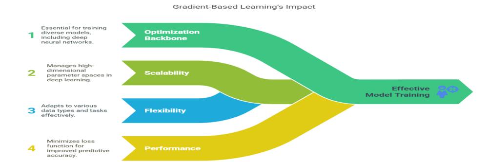
It is fundamental because it allows machine learning models to learn from data effectively and efficiently. Its importance stems from several factors:

• Optimization Backbone: It underpins the training of many models, including linear regression, logistic regression, and especially deep neural networks.
• Scalability: It can handle high-dimensional parameter spaces typical in deep learning.
• Flexibility: It adapts to various types of data and tasks, from image classification to natural language processing.
• Performance: By minimizing the loss function, models generalize better to unseen data, improving predictive accuracy.

Without gradient-based learning, modern AI applications like voice recognition, computer vision, and stock market prediction would be far less feasible.

The Role of Gradient Descent

Gradient descent is the primary algorithm that drives gradient-based learning. It is an iterative optimization method that updates model parameters to minimize the loss function. The process involves:

1. Calculating the Gradient: Compute the derivative of the loss function with respect to each parameter to find the direction of steepest ascent.
2. Parameter Update: Adjust parameters by moving them a small step in the opposite direction of the gradient, scaled by a hyperparameter called the learning rate.
3. Iteration: Repeat these steps until the loss converges to a minimum or stops improving significantly.

Types of Gradient Descent

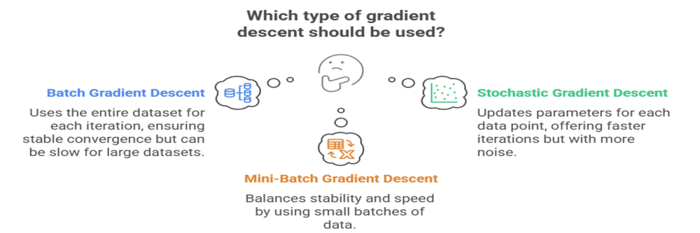
Gradient descent, a key optimization algorithm in machine learning, comes in three main types, each with distinct characteristics and trade-offs:

Batch Gradient Descent

This method computes the gradient of the loss function using the entire training dataset before updating the model parameters. 

It offers stable and accurate convergence but can be computationally expensive and slow for large datasets since it requires processing the full dataset in each iteration (epoch). It often converges smoothly but may get stuck in local minima in non-convex problems.

Stochastic Gradient Descent (SGD)

Instead of using all data points, SGD updates model parameters after evaluating each individual training example. This leads to faster but noisier updates, which can help escape local minima and saddle points but may cause the loss to fluctuate and not converge exactly. 

SGD is memory-efficient since it only needs one data point at a time but can be less stable than batch gradient descent.

Mini-Batch Gradient Descent

Mini-batch gradient descent strikes a balance by dividing the dataset into small batches (e.g., 32 to 256 samples) and updating parameters after each batch. This approach combines the computational efficiency and noise benefits of SGD with the stability of batch gradient descent. It is the most commonly used variant in practice, especially for training deep neural networks.

The mathematical update rule for a parameter θθ is:

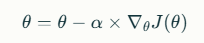
Alt Text: Image showing the mathematical formula for a parameter θθ 

where αα is the learning rate and ∇θJ(θ)∇θJ(θ) is the gradient of the loss function with respect to θθ.

How the Learning Process Works

The learning process can be likened to a hiker descending a mountain to find the lowest valley:

• The hiker starts at a random point (initial parameter values).
• At each step, the hiker looks around to find the steepest downward slope (the gradient).
• The hiker takes a step proportional to the steepness of the slope (learning rate times gradient).
• This process repeats until the hiker reaches the bottom of the valley (minimum loss).

In practice, the model starts with random weights and biases and iteratively updates them based on the gradient of the loss function. Each update moves the model closer to the optimal parameters that minimize prediction error.

Implementation Example

In linear regression, the mean squared error (MSE) is often used as the cost function. The gradient descent algorithm calculates the derivative of MSE with respect to weights and biases, then updates these parameters iteratively. This process continues until the cost function converges or reaches a stopping threshold.

Learning Rate and Convergence

The learning rate (αα) is a critical hyperparameter that determines the size of the steps taken during gradient descent. Its choice significantly affects the training process:

• High Learning Rate: Speeds up convergence but risks overshooting the minimum or causing divergence.
• Low Learning Rate: Ensures stable but slow convergence, increasing training time.
• Adaptive Learning Rates: Methods like Adam, RMSprop, and momentum dynamically adjust the learning rate during training to improve convergence speed and stability.

Choosing an appropriate learning rate is essential to avoid problems such as oscillations around minima or getting stuck in local minima.

Applications of Gradient-Based Learning

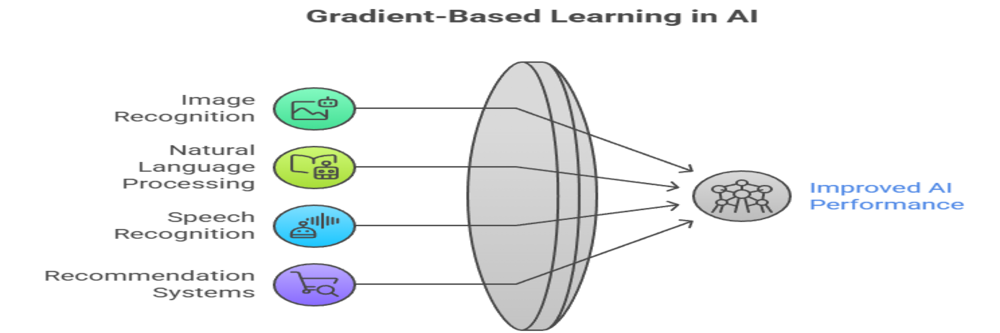
It drives many powerful machine learning applications by optimizing model parameters to minimize errors. It enables breakthroughs in image recognition, natural language processing, speech recognition, and recommendation systems. This section explores how gradient-based methods power diverse AI tasks, improving accuracy and efficiency across industries.

• Deep Neural Networks: Training convolutional neural networks (CNNs) for image recognition, recurrent neural networks (RNNs) for sequence data, and transformers for natural language processing.
• Regression Models: Optimizing parameters in linear and logistic regression.
• Reinforcement Learning: Updating policies based on gradient estimates.
• Generative Models: Training generative adversarial networks (GANs) and autoencoders for data generation and feature extraction.
• Computer Vision and Speech Recognition: Enabling models to learn complex patterns from visual and audio data.

Its versatility and efficiency make gradient-based learning indispensable in modern AI systems.

Challenges and Limitations

Gradient-based learning, while powerful, faces notable challenges and limitations that impact its effectiveness. These include getting trapped in local minima or saddle points, difficulty tuning learning rates, and issues like vanishing or exploding gradients in deep networks. Understanding these hurdles is crucial for improving and applying gradient methods effectively.

• Local Minima and Saddle Points: Non-convex loss landscapes can trap gradient descent in suboptimal points, hindering model performance.
• Vanishing and Exploding Gradients: In very deep networks, gradients can become too small or too large, impeding effective learning.
• Computational Cost: Large datasets and complex models require significant computational resources and time.
• Hyperparameter Sensitivity: The choice of learning rate, batch size, and other parameters critically affects training success.
• Global vs. Local Minima: Gradient descent may converge to a local minimum rather than the global minimum, especially in highly non-convex problems.

Researchers have developed advanced optimization algorithms and architectural techniques to mitigate these issues, such as adaptive optimizers, batch normalization, and residual connections.

Conclusion

Gradient-based learning, powered by gradient descent optimization, is a foundational technique in machine learning that enables models to learn by minimizing error iteratively. It is essential for training a wide array of models, from simple regressors to complex deep neural networks. 

Understanding its mechanisms, tuning parameters like the learning rate, and being aware of its challenges are crucial for building effective and efficient AI systems.

Frequently Asked Questions

What Is the Difference Between Gradient Descent and Gradient-Based Learning?

Gradient descent is a specific optimization algorithm used within gradient-based learning, which broadly refers to any learning method that uses gradients to update model parameters iteratively.

How Does the Learning Rate Affect Gradient Descent?

The learning rate controls the step size during parameter updates. A rate too high can cause divergence, while too low leads to slow convergence. Proper tuning ensures efficient learning.

Can Gradient-Based Learning Handle Non-Convex Functions?

Yes, but it may get trapped in local minima or saddle points. Techniques like stochastic gradient descent and advanced optimizers help navigate these challenges.