Conditional Formatting in Excel – Make Your Data Speak Visually

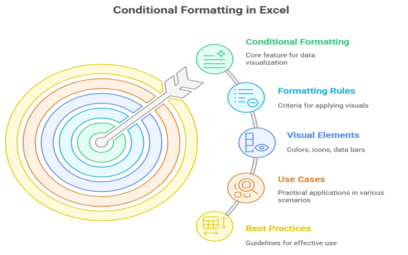
Summary: Conditional formatting in Excel is a powerful feature that automatically applies visual styles to cells based on their values or formulas. It helps users quickly identify trends, outliers, and key information, making data analysis faster and more intuitive. With best practices and practical use cases, anyone can enhance their spreadsheet insights.

Introduction

Conditional formatting in Excel is a powerful feature that transforms raw numbers into meaningful visuals, making your data easier to interpret and analyze. By applying formatting—like colors, icons, or data bars—based on specific rules, you can instantly highlight trends, spot outliers, and draw attention to key information. 

Whether you’re managing sales targets, tracking project deadlines, or analyzing survey results, conditional formatting helps your data speak for itself.

In this comprehensive guide, you’ll learn what conditional formatting is, how to use it, popular use cases, best practices, and solutions to common issues. We’ll also answer frequently asked questions and provide practical, real-world examples for business and personal use.

Key Takeaways

• Instantly highlight important data points with customizable formatting rules.
• Visualize trends and outliers using color scales, data bars, or icons.
• Use formulas for dynamic, context-aware conditional formatting applications.
• Avoid overusing formatting to maintain spreadsheet clarity and effectiveness.
• Regularly review and update rules for optimal performance and accuracy.

How to Apply Conditional Formatting

To apply conditional formatting in Excel, follow these straightforward steps to visually enhance your data and make key information stand out:

Step 1: Select Your Data Range

Highlight the cells, column, table, or entire sheet where you want to apply conditional formatting.

Step 2: Access Conditional Formatting

Go to the Home tab on the Excel ribbon and click Conditional Formatting in the Styles group.

Step 3: Choose a Rule Type

For common scenarios, hover over Highlight Cells Rules or Top/Bottom Rules and pick an option like “Greater Than,” “Less Than,” “Between,” or “Duplicate Values”.

• For visualizations, select Data Bars, Color Scales, or Icon Sets to add graphical elements based on values.
• For custom logic, click New Rule and define your own criteria, including using a conditional formatting Excel formula for advanced needs.

Step 4: Set Your Criteria and Formatting

Enter the specific value, range, or formula that defines when the formatting should apply. Choose your preferred formatting style, such as cell fill color, text color, or icon.

Step 5: Apply and Review

Click OK to apply the rule. Excel will instantly preview the formatting. If satisfied, confirm and close the dialog.

Step 6: Manage or Edit Rules (Optional)

To adjust, remove, or prioritize rules, go to Conditional Formatting > Manage Rules. Here, you can edit, delete, or reorder rules to control which formatting takes precedence.

Tip

You can apply multiple rules to the same range. Use the Rules Manager to arrange their order and set “Stop If True” if you want only the first matching rule to apply.

Example

To highlight salaries above $5,000 in green:

• Select the salary column.
• Go to Home > Conditional Formatting > Highlight Cells Rules > Greater Than.
• Enter 5000, choose a green fill, and click OK.

Conditional formatting is flexible—use it to highlight trends, flag outliers, or make your spreadsheets more readable and actionable.

Popular Use Cases for Conditional Formatting

Conditional formatting in Excel is invaluable for making data-driven decisions and quickly spotting critical information. Here are some of the most popular and practical ways this feature is used:

Highlighting Values Above or Below a Threshold

You can instantly identify numbers that exceed or fall short of a specific value—such as sales above a target or expenses below a budget. For example, highlight employees who sold more than 140 units last year to recognize top performers.

Tracking Dates and Deadlines

Conditional formatting helps monitor upcoming events or overdue tasks. For instance, you can shade cells when a customer’s birthday is within ten days, or flag overdue project deadlines, ensuring timely follow-ups and efficient workflow management.

Detecting Duplicates

Spotting duplicate entries is crucial for data integrity. Use conditional formatting to highlight repeated values in lists, such as duplicate customer IDs or email addresses, so you can clean up your data quickly.

Visualizing Data with Color Scales and Data Bars

Color scales and data bars turn columns of numbers into visual gradients or bars, making it easy to compare values at a glance. This is especially useful for financial analysis, where you might want to visualize revenue growth or expense proportions.

Identifying Top or Bottom Performers

Highlight the top 10% of students in a class, the bottom 5 sales months, or any other ranking-based analysis. Conditional formatting can automatically flag these outliers, helping you focus on the best and worst performers

How to Use Conditional Formatting as a Data Analysis Tool

Conditional formatting in Excel is a powerful data analysis tool that helps you visually interpret large datasets, highlight key trends, and quickly identify outliers or important values. By automatically applying colors, icons, or data bars based on your specified rules, you can transform raw numbers into actionable insights and make your spreadsheets far more intuitive to read and analyze.

Highlighting Key Data Points

Conditional formatting allows you to emphasize cells that meet certain criteria, such as sales figures above a target or expenses below a threshold. For example, you can highlight all sales above $2,500 in green, making it easy to see which team members met their targets without manual review.

Visualizing Trends and Patterns

Using color scales, data bars, or icon sets, you can create instant visualizations that reveal trends, such as increasing or decreasing sales over time, or compare values across categories. These visual cues help you spot patterns and correlations at a glance, which is essential for effective data analysis.

Identifying Outliers and Anomalies

Conditional formatting can automatically flag outliers or errors, such as exceptionally high or low values, or negative numbers. This makes it easy to identify potential issues, data entry mistakes, or exceptional performance that may require further investigation.

Comparing Against Dynamic Benchmarks

You can use conditional formatting formulas to compare each cell’s value to dynamic benchmarks, such as the group average or a changing target. For instance, highlight all sales above the current average using a formula-driven rule. When the benchmark changes, the formatting updates automatically, keeping your analysis current without extra work.

Enhancing Data-Driven Decision-Making

By making important information stand out visually, conditional formatting streamlines data-driven decision-making. Whether you’re tracking project deadlines, monitoring financial KPIs, or analyzing survey results, this feature ensures that critical insights are always visible and easy to act on.

How to Use Conditional Formatting as a Data Analysis Tool

Conditional formatting in Excel is a robust data analysis tool that enables you to visually highlight trends, outliers, and key information by automatically applying formatting based on cell values or formulas. This approach not only enhances the readability of your data but also helps you make faster, more informed decisions by drawing attention to what matters most.

Highlighting Key Data Points

Conditional formatting lets you emphasize cells that meet specific criteria, such as sales figures above a target or expenses below a budget. For example, you can highlight all sales above $2,500 in green, making it easy to instantly spot top performers in your dataset.

Visualizing Trends and Patterns

Tools like data bars and color scales provide immediate visual cues about your data’s distribution. Data bars visually represent the magnitude of values within a range, while color scales use gradients to show relative highs and lows, helping you quickly identify trends or clusters without manual calculations.

Identifying Outliers and Anomalies

Conditional formatting can automatically flag outliers—such as exceptionally high or low values—or errors in your data. This is especially useful for quality control, financial analysis, or any scenario where spotting anomalies is critical to your workflow.

Comparing Against Dynamic Benchmarks

By using formulas in conditional formatting, you can compare each cell’s value to dynamic targets, such as an average or a value in another cell. For example, highlight all sales above the group average with a formula-driven rule; as your data changes, the formatting updates automatically, keeping your analysis current.

Enhancing Data-Driven Decision-Making

Conditional formatting streamlines decision-making by making important information stand out visually. Whether tracking project deadlines, monitoring KPIs, or analyzing survey results, this feature ensures that critical insights are always visible and actionable.

Conditional Formatting Best Practices

Applying conditional formatting in Excel can make your data more readable and actionable, but following best practices ensures your spreadsheets remain clear, efficient, and easy to maintain. Here are the top recommendations for using conditional formatting effectively:

Start Simple

Begin with basic rules that address your main needs, such as highlighting values above or below a threshold. Overcomplicating rules can make your spreadsheet confusing and harder to troubleshoot.

Use Consistent and Meaningful Colors

Choose colors that are intuitive and consistent throughout your workbook—for example, green for positive outcomes and red for negative ones. This helps users quickly understand the meaning behind the formatting.

Avoid Overuse

Too many conditional formatting rules can overwhelm users and reduce the impact of your highlights. Use formatting sparingly to draw attention only to the most important data points.

Make Rules Dynamic

Whenever possible, base your rules on cell references or formulas rather than hardcoded values. This makes your formatting adaptable—when the referenced cell changes, your formatting updates automatically, saving time and reducing errors.

Test and Preview Your Rules

Always preview your conditional formatting before finalizing it. This helps ensure that your rules work as intended and that the visual cues are clear and effective for your audience.

Conclusion

Conditional formatting in Excel empowers you to transform plain data into actionable insights with just a few clicks. From highlighting sales stars to flagging overdue tasks, it’s an essential tool for anyone who works with data. By mastering built-in rules, leveraging formulas, and following best practices, you can make your spreadsheets not just informative, but visually compelling.

Ready to take your Excel skills to the next level? Consider enrolling in our comprehensive Excel training course, where you’ll learn advanced conditional formatting techniques, data analysis strategies, and much more. Unlock the full potential of your data today!

Frequently Asked Questions

How To Use Conditional Formatting in Excel?

Select your data range, go to the Home tab, click Conditional Formatting, choose a rule (e.g., Highlight Cells Rules > Greater Than), set your criteria, and pick a formatting style. Click OK to apply.

What Is the Conditional Formula in Excel?

A conditional formula in Excel is a logical expression (e.g., =A1>100) used to determine whether a cell meets certain criteria. In conditional formatting, the formula must return TRUE (to apply formatting) or FALSE (to leave it unchanged).

How To Use IF With 2 Conditions in Excel?

You can use the AND or OR functions with IF for multiple conditions. Example:
=AND(A1>100, B1=”Yes”)
This formula returns TRUE only if A1 is greater than 100 and B1 equals “Yes”. Use this in a conditional formatting rule to format cells meeting both conditions.