20 Basic Excel Formulas List

Summary: Discover 20 essential Excel formulas designed to boost your productivity and data analysis skills. This guide covers everything from basic calculations like SUM and AVERAGE to powerful lookups like XLOOKUP and logical functions like IF. Master these to save time, reduce errors, and work more efficiently.

Introduction

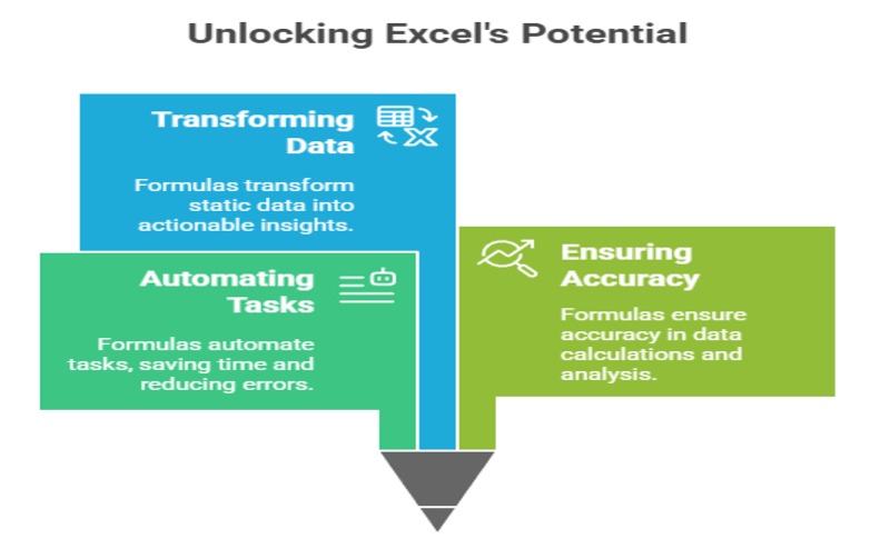
In a world overflowing with data, Microsoft Excel remains a titan of data management and analysis. From organizing a simple shopping list to performing complex financial modeling, its power is undeniable. But the real secret to unlocking Excel’s potential lies within its formulas.

These expressions are the engine that automates tasks, ensures accuracy, and transforms rows of static data into dynamic, actionable insights.

Key Takeaways

1. Master core formulas like SUM, AVERAGE, and COUNT for quick calculations.
2. Use the IF function to make decisions and automate workflow logic.
3. Find specific data in large tables quickly with VLOOKUP or XLOOKUP.
4. Clean and combine text easily using functions like TRIM and CONCAT.
5. Handle formula errors gracefully with IFERROR and use cell references efficiently.

Why Excel Formulas Matter

Excel formulas are the cornerstone of efficiency and precision. They are critical for automating repetitive calculations, which not only saves you a significant amount of time but also drastically reduces the risk of manual errors. Learning to use formulas is more than a technical skill; it’s about empowering yourself to work smarter.

Whether you are a student, a business professional, or managing your personal finances, mastering these basic formulas will fundamentally improve your productivity and your ability to make data-informed decisions.

Excel Formulas You Should Know

Move beyond simple data entry and unlock Excel’s true potential with these essential formulas. Mastering these key functions is the first step to automating your workflow, saving significant time, reducing errors, and transforming how you work with data every day.

1. SUM

The most-used formula in Excel. It adds up all the numbers in a selected range of cells.

• Syntax: =SUM(A2:A10)
• Use Case: Quickly calculate the total sales, expenses, or any list of numbers.

2. AVERAGE

Calculates the arithmetic mean of a range of numbers.

• Syntax: =AVERAGE(B2:B10)
• Use Case: Find the average score of a test, average monthly rainfall, or average product rating.

3. COUNT

Counts the number of cells in a range that contain numbers. It ignores text and empty cells.

• Syntax: =COUNT(C2:C20)
• Use Case: Determine how many sales transactions were made or how many students took an exam.

4. MAX

Finds the highest or maximum value in a range of cells.

• Syntax: =MAX(D2:D100)
• Use Case: Identify the top sales figure, the highest temperature recorded, or the most expensive item on a list.

5. MIN

The opposite of MAX, this function finds the lowest or minimum value in a range.

• Syntax: =MIN(D2:D100)
• Use Case: Find the lowest price, the fastest time in a race, or the smallest measurement.

6. IF

The ultimate logical function. It checks if a condition is true or false and returns a specific value for each outcome.

• Syntax: =IF(logical_test, value_if_true, value_if_false)
• Example: =IF(A2>50, “Pass”, “Fail”) will return “Pass” if the score in A2 is over 50, and “Fail” otherwise.

7. COUNTIF

Counts the number of cells within a range that meet a single, specific criterion.

• Syntax: =COUNTIF(range, criteria)
• Example: =COUNTIF(B2:B20, “London”) will count how many times the word “London” appears in that range.

8. SUMIF

Adds the cells in a range that meet a specific criterion.

• Syntax: =SUMIF(range, criteria, [sum_range])
• Example: =SUMIF(A2:A10, “Fruit”, B2:B10) will sum the values in column B for every row where column A contains “Fruit”.

9. COUNTA

Unlike COUNT, this function counts the number of cells in a range that are not empty, including those with text, numbers, or errors.

• Syntax: =COUNTA(A1:A100)
• Use Case: Quickly see how many items are on a list, even if they are text-based.

10. VLOOKUP

The classic ‘Vertical Lookup’ function. It searches for a value in the first column of a table and returns a corresponding value from another column in the same row.

• Syntax: =VLOOKUP(lookup_value, table_array, col_index_num, [range_lookup])
• Use Case: Find the price of a product by looking up its product ID in a table.

11. XLOOKUP

The modern, more powerful, and flexible successor to VLOOKUP and HLOOKUP. It’s easier to use and overcomes many of their limitations.

• Syntax: =XLOOKUP(lookup_value, lookup_array, return_array)
• Use Case: A superior way to find related data without the column-counting or sorting restrictions of VLOOKUP.

12. INDEX & MATCH

Before XLOOKUP, this combination was the pro’s choice for advanced lookups. INDEX returns a value from a table based on a row and column number, while MATCH finds the position of a lookup value. Together, they are incredibly flexible.

• Syntax: =INDEX(array, MATCH(lookup_value, lookup_array, 0))
• Use Case: Perform complex lookups that can pull data from columns to the left of the lookup column.

13. CONCATENATE (or CONCAT)

Joins text from two or more cells into one.

• Syntax: =CONCAT(A2, ” “, B2)
• Use Case: Combine a first name in one column and a last name in another to create a full name.

14. TRIM

Removes all extra spaces from text, leaving only single spaces between words.

• Syntax: =TRIM(A2)
• Use Case: Clean up data imported from other systems that may have inconsistent spacing.

15 & 16. UPPER & LOWER

            Convert all letters in a text string to uppercase or lowercase, respectively.

• Syntax: =UPPER(A2) or =LOWER(A2)
• Use Case: Standardize text entries for consistent data analysis.

17 & 18. LEFT & RIGHT

Extract a specific number of characters from the beginning (LEFT) or end (RIGHT) of a text string.

• Syntax: =LEFT(text, num_chars) or =RIGHT(text, num_chars)
• Use Case: Extract the first three letters of a product code or the last four digits of a phone number.

19. TODAY()

Returns the current date. This formula is dynamic and will update every time the workbook is opened.

• Syntax: =TODAY()
• Use Case: Create a dashboard that always shows today’s date or calculate project days remaining.

Error Handling

Formulas don’t always work perfectly. This function helps you manage errors gracefully.

20. IFERROR

Checks if a formula evaluates to an error and returns a custom value or message if it does.

• Syntax: =IFERROR(formula, value_if_error)
• Example: =IFERROR(A2/B2, “Invalid Calculation”) will prevent the ugly #DIV/0! error and show your message instead.

Tips for Using Formulas Efficiently

Use Cell References

Instead of typing values directly into formulas (e.g., =5+10), refer to the cells containing those values (e.g., =A1+A2). This makes your formulas dynamic; if the data in the cells changes, the result automatically updates.

The Formula Bar

You can enter and edit formulas directly in a cell or in the formula bar located just above the worksheet grid.

Drag to Fill

Once you’ve written a formula, you can click the small square at the cell’s bottom-right corner (the fill handle) and drag it down or across to copy the formula to other cells.

Absolute vs. Relative References

By default, cell references are relative. When you copy a formula, these references adjust. To lock a reference to a specific cell, use a dollar sign ()tomakeitabsolute(e.g.,‘) to make it absolute (e.g., `)tomakeitabsolute(e.g.,‘A$1`).

Frequently Asked Questions

What is an Excel formula?

An Excel formula is an expression used to perform calculations or manipulate data. It always starts with an equal sign (=) and can include values, cell references, operators (like + or *), and predefined functions (like SUM or IF) to produce a result in a cell.

How do you create a simple formula?

To create a simple formula, select a cell, type an equal sign (=), and then enter your calculation. For example, to add the values in cells A1 and B1, you would type =A1+B1 and press Enter. The cell will then display the calculated result.

What is the difference between a formula and a function?

A formula is any expression in Excel that starts with an equal sign. A function is a pre-built, named formula that simplifies complex calculations. For example, =A1+A2+A3 is a formula, while =SUM(A1:A3) is a formula that uses the SUM function to achieve the same result more efficiently.

How can I see all the formulas in my worksheet?

You can view the formula of any single cell by selecting it and looking at the formula bar. To see all formulas on the worksheet at once instead of their results, you can press the `Ctrl + “ (backtick) key combination. Pressing it again will toggle back to the results view.

Conclusion

Matering this basic Excel formulas list is the first step toward true spreadsheet proficiency. These 20 functions are the foundation for automating tasks, ensuring accuracy, and deriving valuable insights from your data. By moving beyond manual entry and embracing the power of formulas, you don’t just become better at Excel—you become more productive and effective in any data-handling role. Start practicing these simple but powerful tools today and watch your efficiency soar.