Understanding Principal Component Analysis in Machine Learning

Summary: Principal Component Analysis (PCA) in Machine Learning is a crucial technique for dimensionality reduction, transforming complex datasets into simpler forms while retaining essential information. This guide covers PCA’s processes, types, and applications and provides an example, highlighting its importance in data analysis and model performance.

Introduction

The domain of Data Science and Machine Learning is growing fast, and businesses are using it more than ever. By 2025, the Machine Learning market is expected to reach $113.10 billion and increase 34.80% annually, reaching $503.40 billion by 2030. 

However, handling large datasets can be challenging. That’s where Principal Component Analysis (PCA) helps. PCA is a technique that simplifies complex data, making it easier to process and analyze while keeping the most critical information. 

This blog will explain what PCA is, how it works, its benefits, and the different types of PCA. I’ll also describe an example of principal component analysis in Machine Learning, which will help beginners and experts understand this powerful tool in Machine Learning. Additionally, I’ll tell you the difference between factor analysis and principal analysis. 

Key Takeaways

• PCA simplifies complex data by reducing dimensions while preserving essential information for analysis.
• Different PCA types—Standard, Incremental, Kernel, and Sparse—cater to various data complexities.
• PCA enhances Machine Learning by improving model performance, reducing noise, and speeding up computations.
• Real-world applications include feature extraction, data visualisation, and noise reduction in AI and analytics.
• Factor Analysis vs. PCA—PCA maximises variance, while Factor Analysis identifies hidden data relationships.

What is Principal Component Analysis in Machine Learning?

Principal Component Analysis (PCA) is a popular technique in Machine Learning that helps simplify complex data. When working with large datasets, many variables (or features) can make it hard to analyse and visualise the data. 

The PCA algorithm in Machine Learning reduces the number of variables while keeping the most crucial information. This makes data easier to understand and process.

PCA identifies principal components—new variables that summarise the original data. These components are:

• First Principal Component – Captures the most essential patterns in the data.
• Second Principal Component – Captures the most crucial pattern but does not overlap with the first.
• Other Principal Components – Continue capturing patterns, but each adds less information.

These principal components are arranged in a way that retains the most useful information while removing noise and redundancy. Businesses and researchers use PCA to visualise data, remove unnecessary details, and improve Machine Learning models.

Types of Principal Component Analysis

PCA helps transform high-dimensional data into a lower-dimensional space while preserving the essential information. There are various types or variants of PCA, each with its specific use cases and advantages. In this explanation, we’ll cover four main types of PCA:

Standard PCA

Standard PCA is the most common type. It finds patterns in data by identifying key directions (called principal components) that capture the most variation. These components are ranked based on how much information they retain. Standard PCA works well for structured data but may not handle complex patterns efficiently.

Incremental PCA

Incremental PCA is useful for handling large datasets that don’t fit into memory. Instead of processing all data simultaneously, it works on smaller parts in batches. This method reduces memory usage and speeds up calculations, making it ideal for massive datasets.

Kernel PCA

Kernel PCA helps when data has complex, nonlinear patterns. It transforms data into a higher dimension where regular PCA can work more effectively. This method recognises hidden patterns and relationships in datasets that standard PCA might miss.

Sparse PCA

Sparse PCA selects only a few key features from the data, creating a simpler, more focused representation. It is helpful when only certain features matter, making it easier to interpret the results. This method is useful in fields like genetics and finance, where identifying key factors is crucial.

Each type of PCA has strengths and weaknesses, and the choice of variant depends on the dataset’s specific characteristics and the problem at hand.

Process of Principal Component Analysis 

PCA captures the maximum variance in the data by transforming the original variables into a new set of uncorrelated variables called principal components. The process involves several key steps, each crucial for achieving an effective data transformation.

Data Preprocessing

The first step in PCA is data preprocessing, which involves standardizing or normalizing the data. This step ensures that all features have the same scale, as PCA is sensitive to the scale of the features. For instance, if the dataset contains features with different units (e.g., weight in kilograms and height in centimeters), the feature with the larger scale could dominate the principal components. 

Standardisation involves subtracting and dividing the mean by the standard deviation for each feature, resulting in a dataset with a mean of zero and a standard deviation of one. This process ensures that each feature contributes equally to the analysis.

Covariance Matrix Calculation

Once the data is standardised, the next step is to calculate the covariance matrix. The covariance matrix captures the relationships between pairs of variables in the dataset. Precisely, the covariance between two variables measures how much they change together. 

A positive covariance indicates that the variables increase or decrease together, while a negative covariance indicates an inverse relationship. The diagonal elements of the covariance matrix represent the variance of each variable. This matrix serves as the foundation for identifying the principal components.

Eigenvalue Decomposition

With the covariance matrix in hand, the next step is to perform eigenvalue decomposition. This mathematical process decomposes the covariance matrix into its eigenvectors and eigenvalues. The eigenvectors, also known as principal components, represent the directions of maximum variance in the data. 

The corresponding eigenvalues indicate the amount of variance explained by each principal component. In essence, the eigenvectors define a new coordinate system, and the eigenvalues tell us how much of the original dataset’s variability is captured by each new axis.

Selecting Principal Components

After calculating the eigenvalues and eigenvectors, the next step is to select the principal components to retain. Typically, the eigenvectors are sorted in descending order of their corresponding eigenvalues. This sorting allows us to prioritise the principal elements that explain the most variance in the data. 

The choice of how many components to retain (denoted as KKK) depends on the desired level of explained variance. For example, one might retain enough components to explain 95% or 99% of the total variance. This decision balances dimensionality reduction with the preservation of meaningful information.

Projection onto Lower-Dimensional Space

The final step in PCA is projecting the original data onto the lower-dimensional space defined by the selected principal components. This is achieved by transforming the data points using the top KKK eigenvectors. The result is a new dataset with reduced dimensionality, where each data point is represented as a combination of the principal components. 

This transformed dataset can be used for various purposes, such as visualisation, data compression, and noise reduction. Limiting the number of input features also helps reduce multicollinearity and improve the performance of Machine Learning models.

Remember that PCA is a linear transformation technique, and it might not be appropriate for some nonlinear data distributions. In such cases, nonlinear dimensionality reduction techniques like t-SNE (t-Distributed Stochastic Neighbor Embedding) or autoencoders may be more suitable.

Principal Component Analysis in Machine Learning Example 

Let’s walk through a simple example of Principal Component Analysis (PCA) using Python and the popular Machine Learning library, Scikit-learn. In this example, we’ll use the well-known Iris dataset, which contains measurements of iris flowers along with their species. We’ll perform PCA to reduce the data to two dimensions and visualise the results.

• Import the Libraries 
• Load the Iris Dataset and preprocess the data 
• Perform PCA and select the number of principal components 
• Visualise the reduced data 

The resulting scatter plot will show the data points projected onto the two principal components. Each colour corresponds to a different species of iris flowers (Setosa, Versicolor, Virginica). PCA has transformed the high-dimensional data into a 2D space while retaining the most essential information (variance) in the original data.

Remember that the principal component analysis example above uses a small dataset for illustrative purposes. In practice, PCA is most valuable when dealing with high-dimensional datasets where visualising and understanding the data becomes challenging without dimensionality reduction. 

Additionally, the number of principal components (here, 2) can be adjusted based on the specific use case and the desired variance to be retained.

Factor Analysis Vs Principal Component Analysis

When dealing with large amounts of data, we often find patterns and reduce complexity. Two popular techniques that help with this are Factor Analysis (FA) and Principal Component Analysis (PCA). While both are used to reduce the number of variables in a dataset, they serve different purposes.

What is Principal Component Analysis (PCA)?

PCA is a mathematical method that simplifies data by creating new variables called principal components. These components capture the most essential information while removing unnecessary details. PCA is mainly used for data compression, noise reduction, and visualisation. It focuses on keeping as much variation in the data as possible and does not assume any hidden relationships between variables.

What is Factor Analysis (FA)?

Factor Analysis helps find hidden factors that influence the data. It assumes that some unobservable factors affect multiple variables in the dataset. FA is widely used in psychology, social sciences, and market research to identify patterns in human behaviour, opinions, or survey responses.

The key differences between these two are: 

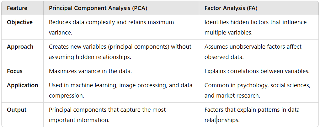
• Objective: PCA reduces data complexity, while FA finds hidden factors behind data relationships.
• Approach: PCA maximises variance, whereas FA looks for underlying patterns.
• Application: PCA is common in image processing and Machine Learning, while FA is used in research and social sciences.

Both techniques are helpful, but choosing the right one depends on the goal of the analysis. I’m including a table highlighting the significant differences between FA and PCA for better understanding. 

Applications of PCA in Machine Learning

PCA simplifies large datasets by reducing the number of features while keeping the most essential information. This helps understand data better, improve Machine Learning models, and make processes more efficient. Here’s how PCA is used in real-world applications:

• Feature Extraction: PCA helps identify the most critical patterns in data, making it easier to analyse.
• Data Visualisation: By reducing complex data to two or three dimensions, PCA makes it possible to create visual representations that reveal hidden trends.
• Noise Reduction: PCA removes unnecessary details (noise) from data, improving accuracy in image and speech recognition tasks.
• Data Compression: It reduces the storage size of datasets without losing critical information, making processing faster.
• Better Machine Learning Performance: By reducing the number of features, PCA speeds up training and improves the efficiency of models used in classification and clustering.

PCA is widely used in fields like finance, healthcare, and marketing, where handling large amounts of data is essential. It simplifies data without losing key insights, making it a necessary technique for better decision-making.

Advantages of PCA in Machine Learning

Principal Component Analysis (PCA) is a powerful tool that helps simplify complex data while retaining essential information. It is widely used in Machine Learning to improve model performance and efficiency. Here are some key advantages of PCA:

• Reduces Dimensionality: PCA minimises the number of features in a dataset, making it easier to process without losing critical information.
• Improves Model Performance: PCA helps Machine Learning models run faster and more efficiently by removing irrelevant or redundant features.
• Enhances Data Visualisation: PCA transforms high-dimensional data into a lower-dimensional space, making it easier to visualise complex patterns.
• Removes Noise: It filters out less essential variations, helping models focus on meaningful data.
• Reduces Overfitting: PCA prevents models from learning unnecessary details, improving generalization.
• Speeds Up Computation: With fewer variables, Machine Learning algorithms run faster, reducing training time.

PCA is a valuable technique for handling large datasets, making data analysis more efficient and insightful.

Disadvantages of PCA in Machine Learning

Principal Component Analysis (PCA) is helpful in simplifying data but has some drawbacks. While it helps reduce complexity, it may not always be the best choice for every situation. Here are some key disadvantages of PCA:

• Loss of Information: Since PCA reduces the number of features, some important details may be lost.
• Hard to Interpret: The new features (principal components) do not have precise meanings, making analysis difficult.
• Not Suitable for Nonlinear Data: PCA works best with linear relationships. If the data has complex patterns, it may not give good results.
• Sensitive to Scaling: PCA requires proper data scaling. If features are not standardised, the results can be misleading.
• Computationally Expensive: For very large datasets, PCA can take a lot of time and resources.

Despite these challenges, PCA is still useful when applied correctly in Machine Learning.

Bottom Line

Principal Component Analysis (PCA) in Machine Learning simplifies large datasets by reducing dimensions while retaining critical information. It enhances data visualisation, improves model performance, and aids feature selection. Different types of PCA cater to various data complexities, making it an essential tool in Data Science. 

While PCA has limitations, such as potential information loss and sensitivity to scaling, it remains a powerful technique for data preprocessing. Understanding PCA’s applications, benefits, and working mechanisms can help businesses and researchers optimise Machine Learning models and extract meaningful insights. Implementing PCA correctly ensures efficient data handling and improved decision-making across multiple domains.

Frequently Asked Questions

What is Principal Component Analysis in Machine Learning?  

Principal Component Analysis (PCA) in Machine Learning is a technique used for dimensionality reduction. It transforms high-dimensional data into a lower-dimensional space, retaining the most critical information by identifying the principal components that capture the maximum variance in the data.

What are the Types of Principal Component Analysis? 

The main types of Principal Component Analysis include Standard PCA, Incremental PCA, Kernel PCA, and Sparse PCA. Each type caters to different data structures and computational needs, such as handling large datasets, nonlinear relationships, or sparse data representations.

How does PCA improve Machine Learning models?

PCA reduces dimensionality, eliminating redundant or irrelevant features. This speeds up computation, prevents overfitting, and enhances accuracy. It also makes high-dimensional data easier to visualise and interpret, improving model training efficiency and enabling better pattern recognition in real-world applications like image processing and financial analysis.