How To Use the INDEX Function in Excel

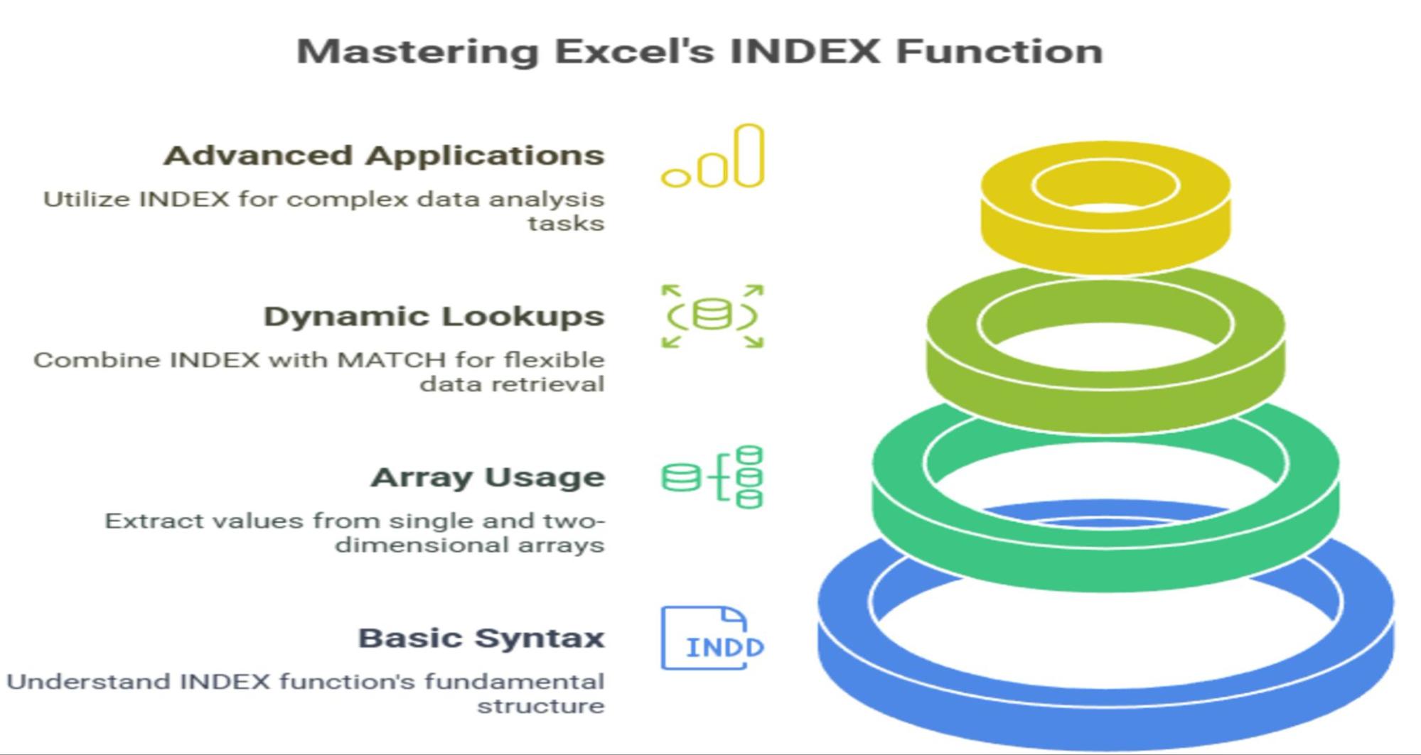
Summary: The INDEX function in Excel returns values by position within arrays or ranges, enabling powerful data extraction. Combined with MATCH, it supports dynamic lookups surpassing VLOOKUP’s limitations. This guide covers syntax, usage, common errors, and practical examples for effective data handling.

Introduction

In today’s data-driven world, Excel remains the most powerful and widely used tool for managing, analyzing, and extracting insights from data. Among the many functions Excel offers, the INDEX function stands out as a versatile and efficient way to extract specific values from your datasets.

Whether you are working with simple lists or complex tables, mastering the INDEX function can significantly enhance your ability to retrieve data accurately and dynamically.

This blog will take you through everything you need to know about the INDEX function in Excel — from its basic syntax and usage with arrays to advanced dynamic lookups with MATCH, comparisons with other lookup functions, common mistakes to avoid, and practical real-world applications.

Key Takeaways

• INDEX retrieves values based on row and column positions.
• MATCH finds lookup positions dynamically for flexible extractions.
• INDEX + MATCH outperforms VLOOKUP in flexibility and speed.
• Avoid errors by checking references and ensuring exact matches.
• INDEX supports one- and two-dimensional array data extraction.

What is the INDEX Function in Excel?

The INDEX function in Excel is designed to return the value or reference of a cell at the intersection of a specified row and column within a given range or array. Unlike lookup functions that search for values based on matching criteria, INDEX works purely by position, which makes it highly efficient and flexible.

Why Use INDEX?

• Precision: You specify the exact row and column position.
• Flexibility: Works with both one-dimensional and two-dimensional arrays.
• Speed: Faster than many lookup functions, especially on large datasets.
• Dynamic: Can be combined with other functions like MATCH for powerful dynamic lookups.
• Versatile: Returns values or references, allowing for complex formulas.

The INDEX function is often paired with the MATCH function to create dynamic, two-way lookups that overcome many limitations of traditional lookup functions like VLOOKUP and HLOOKUP.

Syntax and Parameters of the INDEX Function

The INDEX function has two primary forms: array form and reference form. The array form is most commonly used, so we will focus on that.

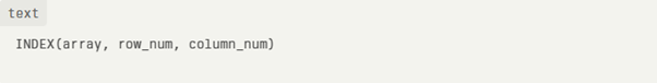
Syntax (Array Form)

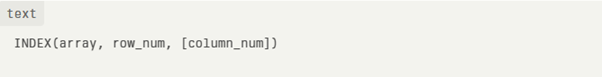
• array (required): The range of cells or array from which you want to retrieve a value.
• row_num (required if column_num is omitted): The row number in the array to return a value from.
• column_num (optional): The column number in the array to return a value from.

Important Notes

• If you provide only row_num for a single-column array, INDEX returns the value in that row.
• If you provide both row_num and column_num for a two-dimensional array, INDEX returns the value at their intersection.
• If row_num or column_num is 0, INDEX returns the entire column or row respectively as an array (available in Excel versions supporting dynamic arrays).
• If the specified row or column is out of range, INDEX returns a #REF! error.

Using INDEX with Single and Two-Dimensional Arrays

Single-Dimensional Array Example

Suppose you have a list of employee names in cells A1:A5:

To retrieve the 3rd name in the list:

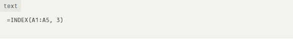
This formula returns Michael, the value in the 3rd row of the range A1:A5.

Two-Dimensional Array Example

Now consider a sales table in range B2:D6:

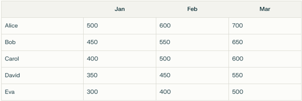
To get the sales figure for Bob in March (row 2, column 3):

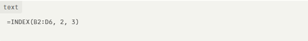
This returns 650, the value at the intersection of the 2nd row and 3rd column in the range.

Dynamic Lookups with INDEX + MATCH

While INDEX retrieves values by position, the MATCH function finds the position of a specific value within a range. Combining these two functions allows you to perform powerful, dynamic lookups that are not limited by the constraints of VLOOKUP or HLOOKUP.

How MATCH Works

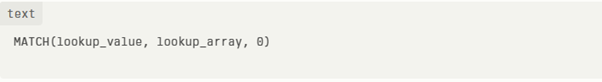
The syntax of MATCH is:

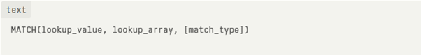
• ookup_value: The value you want to find.
• lookup_array: The range to search.
• match_type: 0 for exact match (recommended for most cases).

MATCH returns the position of the lookup value within the lookup array.

Combining INDEX and MATCH

By using MATCH to find the row and/or column number, and then feeding those into INDEX, you can retrieve values dynamically.

Example: Two-Way Lookup

Using the sales table above, suppose you want to find Carol’s sales in February.

• Find Carol’s row number:

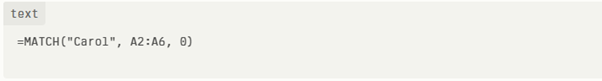
Returns 3 (Carol is the 3rd name in the list).

• Find February’s column number:

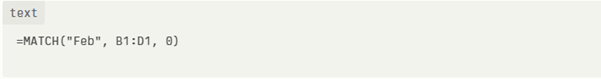
Returns 2 (February is the 2nd column in the range).

• Use INDEX with these results:

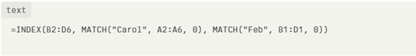
Returns 500, Carol’s sales in February.

Benefits of INDEX + MATCH

• Works with lookup values in any column or row.
• More robust than VLOOKUP (which requires the lookup column to be first).
• Handles large datasets efficiently.
• Supports horizontal and vertical lookups simultaneously.

Comparing INDEX vs. VLOOKUP vs. XLOOKUP

Excel offers multiple lookup functions, each with pros and cons. Understanding how INDEX compares to VLOOKUP and the newer XLOOKUP helps you choose the right tool.

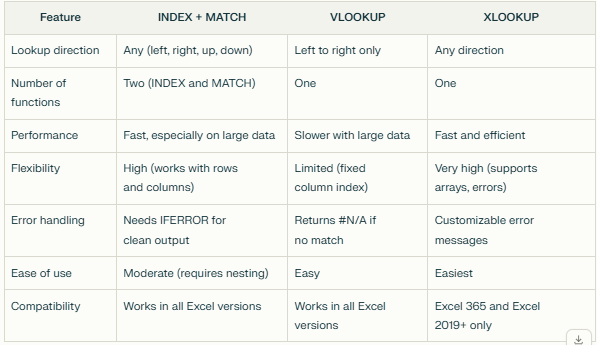
Summary

• VLOOKUP is simpler but limited and less flexible.
• INDEX + MATCH is more powerful and versatile, especially for complex lookups.
• XLOOKUP is the newest and most user-friendly, but requires modern Excel versions.

Common Mistakes and How to Avoid Them When Using the INDEX Function in Excel

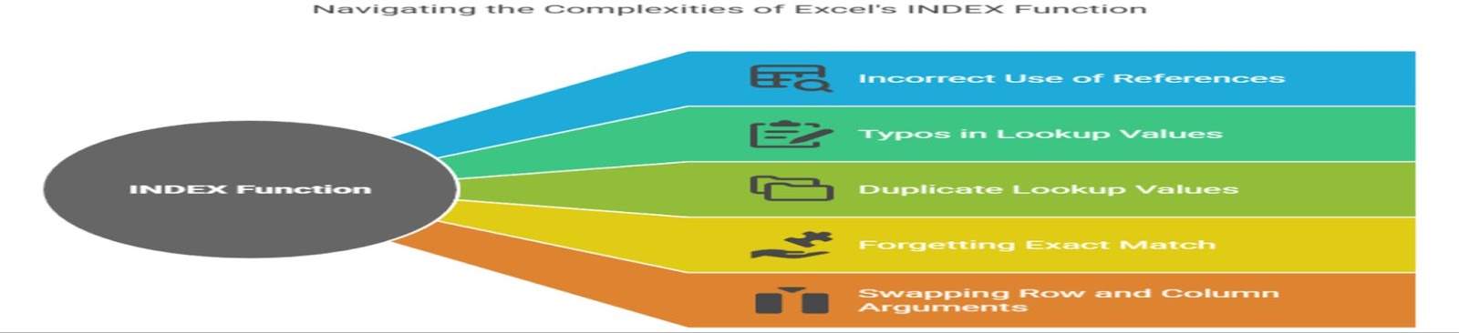
The INDEX function is powerful and flexible, but it can be tricky to use correctly, especially when combined with MATCH. Many users encounter errors or unexpected results due to common pitfalls. Understanding these mistakes and how to avoid them will save you time and frustration.

Incorrect Use of Relative and Absolute References

One of the most frequent errors is improper use of relative and absolute cell references in the formula. When copying or dragging formulas, relative references change, which can cause INDEX or MATCH to reference wrong ranges.

How to avoid

Always use absolute references ($) for your lookup arrays and data ranges when you want them to stay fixed. For example:

Typos in Lookup Values or Lookup Arrays

The MATCH function used inside INDEX requires an exact match (when match_type=0). Even a small typo or extra space in the lookup value or the lookup array can cause the formula to return a #N/A error.

How to avoid

• Double-check spelling and spacing in both your lookup values and lookup arrays.
• Use Excel’s TRIM function to remove extra spaces if necessary.
• Use data validation or dropdown lists to minimize input errors.

Duplicate Lookup Values Causing Unexpected Results

MATCH returns the position of the first occurrence of the lookup value. If your lookup array contains duplicates, INDEX + MATCH will always return the first match, which may not be what you intend.

How to avoid

• Ensure your lookup arrays have unique values.
• If duplicates are unavoidable, consider more advanced formulas or helper columns to distinguish entries.

Forgetting to Specify Exact Match in MATCH Function

The MATCH function’s third argument, match_type, defaults to 1 (approximate match) if omitted. This can cause incorrect results or errors when you expect an exact match.

How to avoid

Always specify 0 as the third argument in MATCH for exact matches:

This prevents unexpected approximate matches and errors.

Swapping Row and Column Arguments in INDEX

A common mistake is reversing the order of the row and column numbers in the INDEX function, especially when using two MATCH functions.

How to avoid

Remember the syntax:

• The first MATCH should find the row number.
• The second MATCH should find the column number.

Swapping these leads to incorrect data retrieval or errors.

Practical Applications of INDEX Function in Excel

The INDEX function in Excel is more than just a tool to retrieve a value from a particular cell in a range; it is a versatile function that can be applied in numerous practical scenarios to enhance data analysis, reporting, and dynamic referencing.

Below, we explore some of the most impactful real-world applications of the INDEX function, supported by examples and explanations.

Extracting Specific Data Points from Tables

One of the most straightforward uses of the INDEX function is to extract a specific value from a table or range based on row and column numbers.

Dynamic Range Creation for Calculations

The INDEX function can return a reference to a cell or range, which can be used dynamically within other functions like SUM, AVERAGE, MAX, or MIN. This allows you to create formulas that adjust automatically based on changing criteria.

Summing Values Between Two Points

You can use two INDEX functions to define dynamic start and end points in a range for summing values.

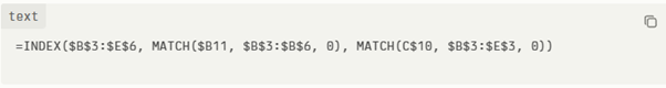
Two-Dimensional Lookups (Row and Column Intersection)

INDEX is ideal for retrieving values at the intersection of a specific row and column, making it perfect for two-way lookups.

Creating Dynamic Dashboards and Reports

Using INDEX with MATCH allows you to build dashboards where users select criteria from drop-down lists, and the displayed data updates automatically.

For instance, selecting a product and month from drop-downs can feed into MATCH functions to find the correct row and column, while INDEX fetches the corresponding data point. This makes reports highly interactive and user-friendly.

Conclusion

The INDEX function is an essential Excel tool that allows you to extract data efficiently by specifying row and column positions. When combined with the MATCH function, it becomes a powerful dynamic lookup tool that surpasses traditional functions like VLOOKUP in flexibility and performance.

Understanding the syntax, common pitfalls, and practical applications of INDEX will empower you to handle complex data retrieval tasks with ease.

Whether you are building dashboards, performing two-dimensional lookups, or automating reports, mastering the INDEX function will make your Excel work more dynamic, accurate, and efficient.

Frequently Asked Questions

What is the Difference Between INDEX and VLOOKUP?

INDEX returns a value based on row and column positions, while VLOOKUP searches for a value in the first column and returns data from a specified column. INDEX + MATCH offers more flexibility and is less prone to errors.

Can INDEX Return Entire Rows or Columns?

Yes. By setting the row_num or column_num to 0, INDEX can return an entire row or column as an array, useful for dynamic reports and advanced formulas.

Why Does My INDEX + MATCH Formula Return #REF! Error?

This error usually means the row or column index is out of range or the ranges in INDEX and MATCH do not align. Double-check your ranges and ensure match_type is set correctly.